ANALYSING EFFECTS OF GLOBAL WARMING ON EARTH USING DATA MINING METHODS
ii
ANALYSING EFFECTS OF GLOBAL WARMING ON EARTH
USING DATA MINING METHODS
A THESIS SUBMITTED TO THE GRADUATE SCHOOL
OF
THE UNIVERSITY of BAHCESEHIR BY
KIVANÇ KILIÇER
IN PARTIAL FULFILLMENT OF THE REQUIREMENTS FOR THE DEGREE OF MASTER OF SCIENCE
IN
THE DEPARTMENT OF INFORMATION TECHNOLOGIES
iii
Approval of the Graduate School of (Name of the Graduate School)
________________ (Title and Name)
Director
I certify that this thesis satisfies all the requirements as a thesis for the degree of Master of Science
___________________ (Title and Name)
Head of Department This is to certify that we have read this thesis and that in our opinion it is fully adequate, in scope and quality, as a thesis for the degree of Master of Science.
_________________ _________________
(Title and Name) (Title and Name) Co-Supervisor Supervisor
Examining Committee Members
... _____________________ ... _____________________ ... _____________________ ... _____________________ ... _____________________
iv
ABSTRACT
ANALYSING EFFECTS OF GLOBAL WARMING ON EARTH USING DATA MINING METHODS
Kılıçer, Kıvanç
M.S. Department of Information Technologies Supervisor: Asst. Prof. Dr. Adem Karahoca
July 2006, 89 pages
In recent years, many geographical and atmospherical incidents are observed on earth because of climate changes, where the global warming has the most important role. The aim of this research is to search the possible effects of global warming on earth and to build a relationship between meteorological variables, by examining the changes from past to today, using data mining methods. Firstly, the climate changes in the past and the attributes behind these changes are determined. For each attribute 70 years daily data is found and the data is merged into a new dataset covering all attributes. Through analyzing the data in computer, correlation coefficients between variables are found for different time periods. As an example, the daily past-values of attributes like sea level, soil moisture and snow depth for different regions on earth are processed in order to understand what kind of anomalities can global warming bring out in the future.
Key Words: Global warming, temperature, soil moisture,
precipitation, data mining, cloud cover, snow depth, climate, glacier, weka, linear regression, humidity
v
ÖZET
KÜRESEL ISINMANIN DÜNYAYA ETKİLERİNİN VERİ MADENCİLİĞİ YÖNTEMİ İLE
ANALİZİ
Kılıçer, Kıvanç
Yüksek Lisans, Bilgi Teknolojileri Bölümü Tez Yöneticisi: Yrd. Doç. Dr. Adem Karahoca
Temmuz 2006, 89 sayfa
Son yıllarda küresel ısınma başta olmak üzere dünyadaki iklim değişiklikleri sebebiyle yerkürede bir çok coğrafi ve atmosferik olaylar gözlenmektedir. Bu çalışmanın amacı, iklim değişikliklerin yer küre üzerindeki olası etkilerini araştırmak ve geçmişten günümüze meteorolojik değişkenlerin değişimini inceleyerek bu değişkenleri veri madenciliği yöntemi ile ilişkilendirmektir. Öncelikle geçmişte gerçekleşen iklim değişiklikleri ve bu değişikliklere yol açan değişkenler saptanmıştır. Bu değişkenlerin 70 yıllık verileri toplanmış ve bu veriler birleştirilerek yeni bir dataset haline getirilmiştir. Datasetlerin bilgisayar ortamında analizi yapılarak çeşitli zaman periyotlarındaki diğer değişkenlerle aralarındaki korelasyon katsayıları çıkartılmıştır. Örneğin, deniz seviyesi, toprak nemliliği, kar kalınlığı gibi değişkenlerin geçmişten günümüze çeşitli bölgelerdeki değerleri toplanarak küresel ısınmanın artışının gelecekte ne gibi etkilere sahip olacağı irdelenmiştir.
Anahtar Kelimeler: küresel ısınma, sıcaklık, toprak nemliliği,
yağış, veri madenciliği, bulut büyüklüğü, kar kalınlığı, iklim, buzul, weka, lineer regresyon, nem
vi
vii
ACKNOWLEDGMENTS
This thesis is dedicated to my wife for her patience and understanding during my master’s study and for her help in the preperation of this thesis. I am also grateful to my mother, who provided moral and spiritual support.
I would like to express my gratitude to Asst. Prof. Dr. Adem
Karahoca, for not only being such a great supervisor but also
encouraging and challenging me throughout my academic program.
viii
TABLE OF CONTENTS
ABSTRACT ... IV TABLE OF CONTENTS ... VIII 1 INTRODUCTION ... 11.1 LITERATURE SURVEY ... 2
2 BASIC CONCEPTS OF CLIMATE CHANGE ... 6
3 OBSERVED CHANGES IN CLIMATE ... 7
3.1 OBSERVED CHANGES IN TEMPERATURE AND PRECIPITATION ... 8
3.2 OBSERVED CHANGES IN SEA LEVEL ... 9
3.3OBSERVED CHANGES IN SEA ICE EXTENT AND CONCENTRATION ... 12
3.4 OBSERVED CHANGES IN OZONE ... 16
4 DETECTION AND ATTRIBUTION OF CLIMATE CHANGE SIGNALS ... 17
5 POTENTIAL IMPACTS OF CLIMATE CHANGE ... 18
5.1WATER RESOURCES ... 18
5.2 AGRICULTURE AND FOOD SECURITY ... 19
6 REGIONAL / LOCAL SCALE CLIMATE CHANGE IMPLICATIONS ... 20
6.1 AFRICAN CLIMATE TRENDS AND PROJECTIONS ... 20
6.1.1 Climate Change Scenarios in Africa ... 20
6.2 MIDDLE EAST AND ARID ASIA ... 22
6.2.1 Observed Temperature and Future Projections ... 22
6.2.2 Observed Precipitation and Future Projections ... 22
6.2.3 Water Resources ... 23
6.3 MEDITERRANEAN REGION ... 23
6.3.1 Observed Changes ... 24
6.3.2 Future Projections ... 25
7 THE UNFCCC AND KYOTO PROTOCOL ... 26
7.1 THE UNFCCC ... 26
7.2 THE KYOTO PROTOCOL ... 27
7.3RECENT CLIMATE CHANGE DEBATES ... 28
8 DEVELOPING AND APPLYING SCENARIOS ... 30
8.1 LAND-USE AND LAND-COVER CHANGE SCENARIOS ... 30
8.1.1 Methods of Scenario Development Future Projections ... 30
8.1.2 Types of Land-Use and Land-Cover Change Scenarios ... 33
8.1.3 Application of Scenarios and Uncertainties ... 36
8.2 ENVIRONMENTAL SCENARIOS ... 41
8.2.1 CO2 Scenarios ... 41
8.2.2 UV-B Radiation Scenarios ... 43
8.2.2 Scenarios of Marine Pollution ... 45
8.3SEA-LEVEL RISE SCENARIOS ... 46
8.3.1 Global Average Sea-Level Rise ... 46
8.3.2 Regional Sea-Level Rise ... 47
8.3.3 Scenarios Incorporating Variability ... 48
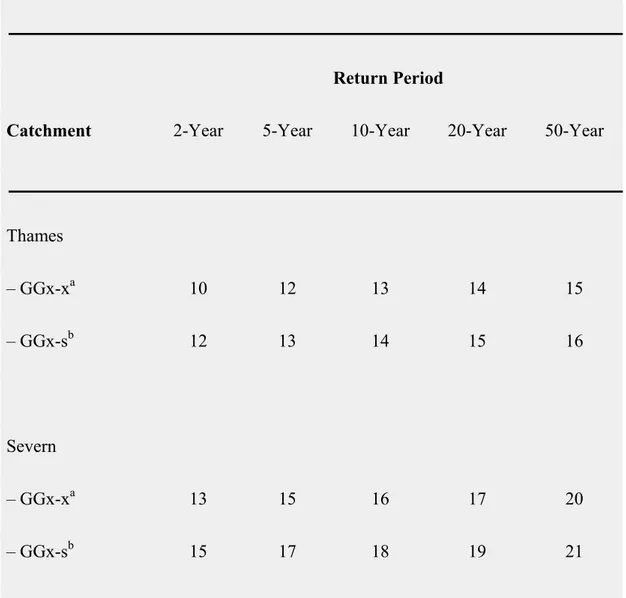
8.4FLOOD SCENARIOS ... 50
8.4.1 Changes in Flood Frequency ... 50
ix
9.1 DATA MINING METHOD ... 52
9.2 DATA MINING SOFTWARE: WEKA ... 53
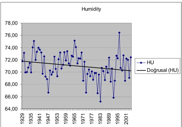
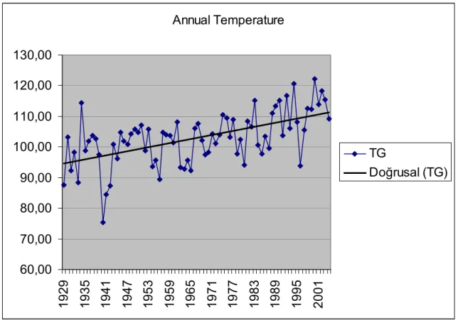
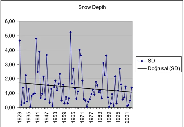
9.3DATASETS ... 54 9.3.1 Humidity ... 55 9.3.2 Mean Temperature ... 55 9.3.3 Cloud Cover ... 56 9.3.4 Precipitation ... 56 9.3.5 Snow Depth ... 57 9.3.6 Sunshine ... 57
9.4 DATASET COMBINATION AND GROUPING ... 58
9.5 FINAL DATASET ... 60
9.6 BASIC RELATIONSHIP BETWEEN ATTRIBUTES ... 60
9.7PROCESSING AND VISUALIZING ALL ATTRIBUTES IN WEKA ... 64
9.7.1 Discretisizing ... 65 9.7.2 Classification ... 66 9.7.3 Clustering Method ... 80 9.7.4 Prediction ... 83 10 CONCLUSION ... 84 REFERENCES ... 86 VITA ... 89
1
1 INTRODUCTION
On a global scale, there is increasing evidence that climate is changing. Increased concentrations of greenhouse gases in the atmosphere due to human activities are believed to be the underlying cause of the change in global climate. The atmospheric concentrations of greenhouse gases, mainly carbon dioxide (CO2), methane (CH4) and nitrous oxide (N2O), have risen significantly since the pre-industrial era. Current estimates indicate that the CO2 concentrations in the atmosphere have reached to almost 370 ppmv3, which is a 30 percent increase from its pre-industrial levels. (Keeling, Ralph, Stephen Piper, Martin Heimann, 1996) The model simulations indicate that global average surface temperatures will rise by 1.5-4.5°C over the next 100 years assuming that no action is taken to reduce emissions. Scientists expect that the average global surface temperature could rise 1-4.5°F (0.6-2.5°C) in the next fifty years, and 2.2-10°F 1.4-5.8°C) in the next century, with significant regional variation. Instrumental temperature records provide some evidence that the warming is already begun. Average world surface temperatures appear to have risen by 0.3-0.6°C over the past 100 years. The warming is even more prominent in the last three decades. The global average surface temperature in 2001 was the second warmest on record, 0.42°C above the 1961-1990 average. Some climatologists, however, believe that these observed warming is still within the range of natural variability. (Information Unit on Climate Change, 2001)
Rising global temperatures are expected to raise sea level, and change precipitation and other local climate conditions. Changing regional climate could alter forests, crop yields, and water supplies. It could also affect human health, animals, and
2
many types of ecosystems. Evaporation will increase as the climate warms, which will increase average global precipitation. Soil moisture is likely to decline in many regions, and intense rainstorms are likely to become more frequent.
1.1 Literature Survey
Climate change issue has been observed and projected in the past studies. Some examples of these studies are as follows:
1) “Probabilistic Climate Change Projections Using Neural Networks”
The research presents a neural network based climate model substitute that increases the efficiency of large climate model ensembles by at least an order of magnitude. Using the observed surface warming over the industrial period and estimates of global ocean heat uptake as constraints for the ensemble, this method estimates ranges for climate sensitivity and radiative forcing that are consistent with observations. In particular, negative values for the uncertain indirect aerosol forcing exceeding -1.2 W m[-2] can be excluded with high confidence. A parameterization to account for the uncertainty in the future carbon cycle is introduced, derived separately from a carbon cycle model. This allows us to quantify the effect of the feedback between oceanic and terrestrial carbon uptake and global warming on global temperature projections. Finally, probability density functions for the surface warming until year 2100 for two illustrative emission scenarios are calculated, taking into account uncertainties in the carbon cycle, radiative forcing, climate sensitivity, model parameters and the observed temperature records. The research finds that warming exceeds the surface warming range projected by IPCC for almost half of the ensemble members. Projection uncertainties are only consistent with
3
IPCC if a model-derived upper limit of about 5 K is assumed for climate sensitivity. (Knutti R., Stocker T. F., Joos F., Plattner G.-K., 1986)
2) “Rainfall Forecasting Using Soft Computing Models and Multivariate Adaptive Regression Splines”
Long-term rainfall prediction is a challenging task especially in the modern world where we are facing the major environmental problem of global warming. In general, climate and rainfall are highly non-linear phenomena in nature exhibiting what is known as the "butterfly effect". While some regions of the world are noticing a systematic decrease in annual rainfall, others notice increases in flooding and severe storms. The global nature of this phenomenon is very complicated and requires sophisticated computer modeling and simulation to predict accurately. The past few years have witnessed a growing recognition of Soft Computing (SC) technologies that underlie the conception, design and utilization of intelligent systems . In this paper, the SC methods considered are
i) Evolving Fuzzy Neural Network (EFuNN)
ii) Artificial Neural Network using Scaled Conjugate Gradient Algorithm iii) Adaptive Basis Function Neural Network (ABFNN) and
iv) General Regression Neural Network (GRNN).
Multivariate Adaptive Regression Splines (MARS) is a regression technique that uses a specific class of basis functions as predictors in place of the original data. In this paper, it is reported a performance analysis for MARS and the SC models considered. To evaluate the prediction efficiency, 87 years of rainfall data in Kerala state, the southern part of the Indian peninsula is used. (Abraham A.., Steinberg D., Philip N., 2001)
4
3) “Neural Network Modeling of Climate Change Impacts on Irrigation Water Supplies in Arkansas River Basin”
Climate change in the region that includes the Arkansas River basin may have profound effects on water users. The potential impacts of climate change include changes in snowfall, snowmelt and rainfall amount and intensities. Snowmelt is the main source of water supply in the region. Water supply is a key factor in determining agricultural potential. In scientific studies dealing with modeling irrigation water budgets, water supply is usually assumed sufficient. The possible effects of climatic changes on surface water supplies for irrigation in the Arkansas River basin are investigated using Artificial Neural network (ANN). ANN models have been found useful and efficient, particularly in problems for which the characteristics of the process are difficult to describe using physically based models. ANN is capable of identifying complex nonlinear relationships between input and output data sets without prior knowledge of the internal structure of a system. This study presents a procedure for modeling the impacts of climate change on irrigation water supplies and demonstrates the potential of ANN models for simulating such nonlinear hydrologic behavior. Precipitation over the mountains and the basin area coupled with steam flow is used to quantify the impacts of climate changes on surface water supply for irrigation. A feedforward neural network is trained to map the relation between the water diverted for irrigation (output) and the streamflow/precipitation (inputs).
The Research projects an increase in temperature (4 – 7o C) and winter precipitation and a decrease in summer precipitation. Based on these projections the study region is expected to get drier. These dry conditions have adverse effects on water supplies
5
in the region. Following the projected precipitation patterns, a decrease in water supply will occur. In 2060 a reduction in water supplies will occur from midseason (April/May) to the end of the season (June-Sept.). In 2090, based on the projections, water will be short over the whole season. High projected temperature increases ET and alters snowmelt time causing a shift in water availability to late winter and early summer. The study region is one of the regions most vulnerable to climate change. Water shortage is already a problem in the region. If precipitation amounts and timing change as projected, the water resources in the region will be under more stress. (Elgaali E., Garcia L., 2002)
6
2 BASIC CONCEPTS OF CLIMATE CHANGE
Climate is the average state of the atmosphere and is typically described by the statistics of a set of atmospheric and surface variables, such as temperature, precipitation, wind, humidity, cloudiness, soil moisture, and sea surface temperature in terms of the long-term average. Although climate and climate change are usually presented in global mean terms, there may be large local and regional departures from these global averages. Factors that contribute to climate and climate change are usually defined by climate forcing. A climate forcing can be defined as an imposed perturbation of Earth’s energy balance. An increase in the luminosity of the sun, for example, is a positive forcing that leads a warmer Earth. A very large volcanic eruption, on the other hand, can increase the aerosols in the lower stratosphere, and thereby reduces the solar energy delivered to Earth’s surface. These examples are natural forcing. Human-made forcing result from, for example, the gases and aerosols produced by fossil fuel burning, and alterations of Earth’s surface from various changes in land use, such as the conversion of forests into agricultural land. The observations of human-induced forcing underlie the current concerns about climate change. (The National Academies Press, “Climate Change Science: An Analysis of Some Key Questions, 2001)
7
3 OBSERVED CHANGES IN CLIMATE
Since 1860, mean global temperatures have risen by between 0.3°C and 0.6°C.Warming since the mid-1970s has been particularly rapid with nine of the ten warmest years have occurred since 1990, including 1999 and 2000 despite cooling influence of the tropical Pacific La Niña which contributed to a somewhat lower global average (0.29°C and 0.26°C above average, respectively).The warming trend is spatially widespread and is consistent with the global retreat of mountain glaciers, reduction in snow-cover extent, the accelerated rate of rise of sea level during the 20th century relative to the past few thousand years, and the increase in upper-air water vapor and rainfall rates over most regions. The ocean, which represents the largest reservoir of heat in the climate system, has warmed by about 0.05°C averaged over the layer extending from the surface down to 10,000 feet, since the 1950s. Sea ice in the central Arctic has thinned since the 1970s. A decline of about 10% in spring and summer continental snow cover extent over the past few decades also has been observed. (IPCC Technical Summary, Climate Change, 2001)
Satellite data on temperatures in the lower 4.8 miles of the atmosphere, spanning a period from 1979 to the present, show little if any warming trend compared with the surface-based record during the same period. However, the 1979-2000 satellite data series may be too short to show a trend in atmospheric temperature. Balloon-borne instruments used to measure temperatures in the lower 4.8 miles of the atmosphere since 1958, show an overall warming trend from 1958-2000 similar to that of the surface record. But when just the period 1979-2000 is considered, the
8
balloon data resemble the satellite data. (US Environmental Protection Agency web site, 2006)
3.1 Observed Changes in Temperature and Precipitation
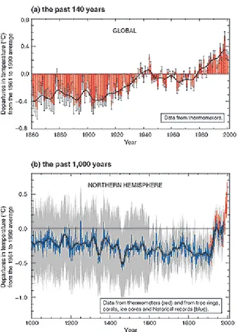
The global average surface temperature has increased by 0.6 - 0.2°C since the late 19th century. It is very likely that the 1990s was the warmest decade and 1998 the warmest year in the instrumental record since 1861. Most of the increase in global temperature since the late 19th century has occurred in two distinct periods: 1910 to 1945 and since 1976. The most recent period of warming (1976 to 1999) has been almost global, but the largest increases in temperature have occurred over the mid- and high latitudes of the continents in the Northern Hemisphere.
Annual land precipitation has continued to increase in the middle and high latitudes of the Northern Hemisphere at a rate of 0.5 to 1% /decade), except over Eastern Asia. Over the sub-tropics (10°N to 30°N), land surface rainfall has decreased on average around 0.3% /decade, although this has shown signs of recovery in recent years. Tropical land-surface precipitation measurements indicate that precipitation likely has increased by about 0.2 to 0.3%/ decade over the 20th century, but increases are not evident over the past few decades and the amount of tropical land (versus ocean) area for the latitudes 10°N to 10°S is relatively small. Nonetheless, direct measurements of precipitation and model predictions indicate that rainfall has also increased over large parts of the tropical oceans. In contrast to the Northern Hemisphere, no comparable systematic changes in precipitation have been detected in broad latitudinal averages over the Southern Hemisphere. (National Academiy Press, 1996)
9
Figure 3.1 Variations of the Earth’s surface temperature over the last 140 years and the last millennium. (UN Environment Program, 2006)
3.2 Observed Changes in Sea Level
Sea level has risen worldwide approximately 15-20 cm in the last century. Approximately 2-5 cm of the rise has resulted from the melting of mountain glaciers. Another 2-7 cm has resulted from the expansion of ocean water that resulted from warmer ocean temperatures. The pumping of ground water and melting of the polar ice sheets may have also added water to the oceans. Based on tide gauge data, the rate of global mean sea level rise during the 20th century is in the range 1.0 to 2.0 mm/yr. Based on the very few long tide-gauge records, the average rate of sea level rise has been larger during the 20th century than during the 19th century. No significant acceleration in the rate of sea level rise during the 20th
10
century has been detected. This is not inconsistent with model results due to the limited data.
Global sea level is currently rising as a result of ocean thermal expansion and glacier melt, both caused by recent increases in global mean temperature. Antarctica and Greenland, the world's largest ice sheets, make up the vast majority of the Earth's ice. If these ice sheets melted entirely, sea level would rise by more than 70 meters.
Although current estimates indicate that mass balance for the Antarctic ice sheet is in approximate equilibrium, the Greenland Ice Sheet may have contributed substantial mass to the ocean due to negative mass balance. Some areas of the Antarctic have shown significant imbalance, e.g., Pine Island, Thwaites, and glaciers in the Antarctic Peninsula. (There is still much uncertainty about accumulation rates in Antarctica, especially the East Antarctic Plateau.)
Global mass balance data are transformed to sea-level equivalent by multiplying annual average mass balance (approximately -190 millimeters for the period 1961 to 2003) by the surface area of these "small" glaciers (785,000 square kilometers). When dividing this value by the surface area of the oceans (361.6 million square kilometers), the final result is 0.4 millimeters of sea level rise per year. The Glacier Contribution to Sea Level graph demonstrates how the contribution to sea level rise from melting glaciers began increasing at a faster rate starting in the late 1980s. This is in agreement with high-latitude air temperature records (US Environmental Protection Agency web site, 2006).
11
Figure 3.2 Glacier Contributions to Sea Level (National Snow and Ice Data Center web site, 2006)
Over the past 100 years, sea level has risen by 1.0 to 2.5 millimeters per year; thus the contribution from melting small glaciers would be approximately 20 to 30 percent of the total. Climate models based on the current rate of increase in greenhouse gases, however, indicate that sea level will rise at a rate of about two to five times the current rate over the next 100 years from the combined effect of ocean thermal expansion and increased glacier melt. Below graph indicates the glacier contribution to sea level vs. annual global air temperature.
12
Figure 3.3 Glacier Contributions to Sea Level and Air Temperature (National Snow and Ice Data Center web site, 2006)
3.3 Observed Changes in Sea Ice Extent and Concentration
Sea ice is important because it regulates exchanges of heat, moisture and salinity in the polar oceans. It insulates the relatively warm ocean water from the cold polar atmosphere except where cracks, or leads, in the ice allow exchange of heat and water vapor from ocean to atmosphere in winter. The number of leads determines
13
where and how much heat and water are lost to the atmosphere, which may affect local cloud cover and precipitation (ENN News Archive, 1998).
The seasonal sea ice cycle affects both human activities and biological habitats. For example, companies shipping raw materials such as oil or coal out of the Arctic must work quickly during periods of low ice concentration, navigating their ships towards openings in the ice and away from treacherous multi-year ice that has accumulated over many years. Many arctic mammals, such as polar bears, seals, and walruses, depend on the sea ice for their habitat. These species hunt, feed, and breed on the ice. Should the sea ice recede excessively, scientists worry that increased nutritional stresses on the limited food chain may adversely affect these populations, particularly polar bears who must store large amounts of fat to survive arctic winters (Environmental News Network 1998).
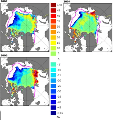
Ice thickness, its spatial extent, and the fraction of open water within the ice pack can vary rapidly and profoundly in response to weather and climate. Sea ice typically covers about 14 to 16 million square kilometers in late winter in the Arctic and 17 to 20 million square kilometers in the Antarctic Southern Ocean. The seasonal decrease is much larger in the Antarctic, with only about three to four million square kilometers remaining at summer's end, compared to approximately seven to nine million square kilometers in the Arctic. The maps below provide examples of late winter and late summer ice cover in the two hemispheres (National Climatic Data Center web site, 2006).
14
Figure 3.4 Arctic and Antarctic sea ice concentration climatology from 1978-2002, at the approximate seasonal maximum and minimum levels. Image provided by National Snow and Ice Data Center, University of Colorado, Boulder. (National Snow and Ice Data Center web site, 2006)
Figure 3.5 Sea ice conditions for September 2002, 2003, and 2004, derived from the Sea Ice Index (National Snow and Ice Data Center web site, 2006)
15
Sea ice thickness has shown substantial decline in recent decades. Using data from submarine cruises, Rothrock and collaborators determined that the mean ice draft at the end of the melt season in the Arctic has decreased by about 1.3 meters over the past 30 to 40 years. These recent trends and variations in ice cover are consistent with recorded changes in high-latitude air temperatures, winds, and oceanic conditions. It is important to note though, that the ice cover responds to a variety of climatic factors, and the available record of sea ice cover is relatively short. (UN Environment Programme, 2006)
Satellite data from the SMMR and SSM/I instruments have also been combined with earlier observations from ice charts and other sources to yield a time series of arctic ice extent from the early 1900s onward.
Figure 3.6 Decrease in Arctic Sea Ice Draft from 1958 to 1997. Graph derived from Rothrock et al. 1999(National Snow and Ice Data Center web site, 2006).
16
3.4 Observed Changes in Ozone
Global monitoring of ozone levels from space by the Total Ozone Mapping Spectrometer (TOMS) instrument has shown statistically significant downward trends in ozone at all latitudes outside the tropics. Measurements at several ground-based stations have shown corresponding upward trends in CFCs in both the northern and southern hemisphere. Ozone depletion and climate change are linked in a number of ways, but ozone depletion is not a major cause of climate change. The climate impact of changes in ozone concentrations varies with the altitude at which these ozone changes occur. The major ozone losses that have been observed in the lower stratosphere due to the human-produced chlorine- and bromine-containing gases have a cooling effect on the Earth's surface. On the other hand, the ozone increases that are estimated to have occurred in the troposphere because of surface-pollution gases have a warming effect on the Earth's surface, thereby contributing to the "greenhouse" effect (Ciesin, Colombia University web site, 2006).
Stratospheric ozone depletion, caused by increasing concentrations of human- produced chemicals, has increased since the 1980s. The springtime loss in Antarctica is the largest depletion. Currently, in nonpolar regions, the ozone layer has been depleted up to several percent compared with that of two decades ago. The magnitude of ozone depletion varies between the regions of the Earth. Since the early 1980s, the ozone hole has formed over Antarctica during every Southern Hemisphere spring (September to November), in which up to 60% of the total ozone is depleted. Since the early 1990s, ozone depletion has also been observed
17
over the Arctic, with the ozone loss from January through late March typically being 20-25% in most of the recent years. WMO 2000 Antarctic Ozone Summary reports an exceptionally large area of very low stratospheric temperatures over Antarctica which set the stage for the earlier than usual development of the annual Austral Spring ozone hole. By early September of 2000, the ozone hole was the largest ever on record, and in late September and early October it was also the deepest. During this period, losses of total column atmospheric ozone exceeded 50 percent within most of the area of the ozone hole (World Meteorological Organization, Global Ozone Research and Monitoring Project, 1998).
4 DETECTION AND ATTRIBUTION OF CLIMATE
CHANGE SIGNALS
The purpose of the climate change detection and attribution activity is to identify variability and trends in the climate system and to ascribe these changes to specific factors, whether natural or man-induced.
The science of detection comprises several key elements: 1) understanding natural change through the paleo record and model simulations; 2) development and implementation of advanced statistical techniques for climate signal identification; and 3) analysis of observations and model output to understand the limitations of both data sources (i.e., uncertainty estimates) and to validate model hind casts of climate system response to natural and anthropogenic forcing. Although temperature is usually the first variable considered in assessments of global climate change, it is important to consider other data that integrate the state of the climate system over space and time. These include temperature proxy data (such as tree
18
ring records), borehole temperature measurements in soil, permafrost, and ice sheets, and measurements of the mass balance of valley glaciers and ice caps. Through analysis of paleo-proxy records (tree rings, ice cores, corals, etc.); past climate variations in the pre-industrial era can be described and used to provide a context for statements about present and future climate possibilities. Besides the long-term data, general circulation models (GCMs) are the major tools in climate change detection and attributions. However, predictions of future climate are imperfect because they are limited by significant uncertainties (Miller C., 2000).
5 POTENTIAL IMPACTS OF CLIMATE CHANGE
Natural and human systems are expected to be influenced by climatic variations such as changes in the average, range, and variability of temperature and precipitation, as well as the frequency and severity of weather events. The following section discusses impacts of climate change on various sectors.
5.1 Water Resources
The effect of climate change on stream flow and groundwater recharge varies regionally and among scenarios, largely following projected changes in precipitation. There are apparent trends in stream flow volumes—increases and decreases—in many regions. However, confidence that these trends are a result of climate change is low because of factors such as the variability of hydrological behavior over time, the brevity of instrumental records, and the response of river flows to factors other than climate change.
19
rain rather than snow and therefore is not stored on the land surface until it melts in spring. In particularly cold areas, an increase in temperature would still mean that winter precipitation falls as snow, so there would be little change in stream flow timing in these regions.
Flood magnitude and frequency are likely to increase in most regions, and low flows are likely to decrease in many regions. Changes in low flows are a function of changes in precipitation and evaporation. Evaporation generally is projected to increase, which may lead to lower flows even where precipitation increases or shows little change. Projected climate change could further decrease stream flow and groundwater recharge in many of these water-stressed countries—for example, in central Asia, southern Africa, and countries around the Mediterranean Sea (IPCC Technical Summary, 2001).
5.2 Agriculture and Food Security
It is established with medium confidence that a few degrees of projected warming will lead to general increases in temperate crop yields, with some regional variation. At larger amounts of projected warming, most temperate crop yield responses become generally negative. In regions where some crops are near their maximum temperature tolerance and where dry land agriculture predominates, yields are expected to decrease generally with even minimal changes in temperature. Also where there is a large decrease in rainfall, crop yields would be even more adversely affected (medium confidence). Higher minimum temperatures will be beneficial to some crops, especially in temperate regions, and detrimental to other crops, especially in low latitudes (high confidence).
20
In arid or semi-arid areas where climate change is likely to decrease available soil moisture, agricultural productivity is expected to decrease. Increased CO2 concentrations may counteract some of these losses. However, many of these areas are affected by El Niño/La Niña, other climatic extremes, and disturbances such as fire. Changes in the frequencies of these events and disturbances could lead to loss of productivity thus potential land degradation, potential loss of stored carbon, or decrease in the rate of carbon uptake (UN Environment Programme, 2006).
6 REGIONAL / LOCAL SCALE CLIMATE CHANGE
IMPLICATIONS
As global climate appears to be changing, we would expect that climate also will change regionally and locally. Detection of climate change on this scale is, however, extremely difficult as the high variability in local climates masks trends in the 'noise' of natural fluctuations. Moreover, the short period of observations makes the identification of clear trends difficult and creates uncertainty over the scale of natural variability. No current climate model is capable of providing realistic regional/ local scale climate change signals. Recent attempts have been made to use nested regional GCMs to down scale global climate change signals to regional levels. Following sections discusses observed and projected climate change for the selected regions where water and agricultural sectors will be affected significantly.
6.1 African Climate Trends and Projections
6.1.1 Climate Change Scenarios in Africa21
over the Sahara and semi-arid parts of southern Africa. Equatorial countries might be about 1.4°C warmer. This projection represents a rate of warming to 2050 of about 0.2°C per decade.
Sea- surface temperatures in the open tropical oceans surrounding Africa will rise by less than the global average (i.e., only about 0.6–0.8°C); the coastal regions of the continent therefore will warm more slowly than the continental interior. Rainfall changes projected by most GCMs are relatively modest, at least in relation to present-day rainfall variability. In general, rainfall is projected to increase over the continent—the exceptions being southern Africa and parts of the Horn of Africa; here, rainfall is projected to decline by 2050 by about 10%. Seasonal changes in rainfall are not expected to be large. Great uncertainty exists; however, in relation to regional-scale rainfall changes simulated by GCMs. Parts of the Sahel could experience rainfall increases of as much as 15% over the 1961–90 average. Equatorial Africa could experience a small (5%) increase in rainfall. These rainfall results, however, are not consistent (Keeling R., Piper S., Heimann, M.,1996).
Projected temperature increases are likely to lead to increased open water and soil/plant evaporation. Exactly how large this increased evaporative loss will be would depend on factors such as physiological changes in plant biology, atmospheric circulation, and land-use patterns. As a rough estimate, potential evapotranspiration over Africa is projected to increase by 5–10% by 2050. Rainfall may well become more intense, but whether there will be more tropical cyclones or a changed frequency of El Niño events remains largely speculated (Marland G..,
22
Pippin A., 1990).
6.2 Middle East and Arid Asia
6.2.1 Observed Temperature and Future Projections
The observed change in annual temperature in the region from 1955–74 to 1975–94 was 0.5°C. Annual temperatures in most of the Middle East region showed almost no change during the period 1901–96, but a 1–2°C/century increase was discernible in central Asia (based on the 5°x5° grid). There was a 0.7°C increase during 1901– 96 in the region as a whole.
Climate models that include the effects of sulfate aerosols (GFDL and CCC) project that the temperature in the region will increase 1–2°C by 2030–2050. The greatest increases are projected for winter in the northeast and for summer in part of the region’s southwest. (UN Environment Programme, 2006)
6.2.2 Observed Precipitation and Future Projections
Rainfall is low in most of the region, but it is highly variable seasonally and interannually. There was no discernible trend in annual precipitation during 1901– 95 for the region neither as a whole nor in most parts of the region— except in the southwestern part of the Arabian Peninsula, where there was a 200% increase. This increase, however, is in relation to a very low base rainfall (<200 mm/yr). Precipitation tends to be very seasonal; in the Middle East countries, for example, precipitation occurs during winter, and the summer dry period lasts for 5–9 months. Winter precipitation is projected to increase slightly (<0.5 mm/day) throughout the region; summer precipitation is projected to remain the same in the northeastern
23
part of the region and increase (0.5–1 mm/day) in the Southwest (i.e., the southern part of the Arabian peninsula). These projected changes vary, however, from model to model and are unlikely to be significant. Soil moisture is projected to decrease in most parts of the region because projected precipitation increases are small and evaporation will increase with rising temperatures.
6.2.3 Water Resources
In an area dominated by arid and semi-arid lands, water is a very limited resource. Droughts, desertification, and water shortages are permanent features of life in many countries in the region. Rapid development is threatening some water supplies through salinization and pollution, and increasing standards of living and expanding populations are increasing demand. Water is a scarce resource—and will continue to be so in the future. Projections of changes in runoff and water supply under climate change scenarios vary. Some countries are developing programs to conserve and reuse water or to achieve more efficient irrigation. (UN Environment Programme, 2006)
6.3 Mediterranean Region
One key finding is that future climate change could critically undermine efforts for sustainable development in the Mediterranean region. In particular, climate change may add to existing problems of desertification, water scarcity and food production, while also introducing new threats to human health, ecosystems and national economies of countries. The most serious impacts are likely to be felt in North African and eastern Mediterranean countries (Marland G.., Pippin A., 1990).
24
6.3.1 Observed Changes
Sea surface temperature records for the Mediterranean region show clear fluctuations in climate over the last 120 or so years, but little overall trend. This record shows that temperatures rose sharply to a maximum around 1940 after which they stabilized for around 20 years. After this, while global temperatures continued to rise to unprecedented levels, the Mediterranean region experienced a decade of rapid cooling. Warming resumed in the late 1970s, but still temperatures remained below those experienced in the 1930s and 1940s up until 1989 at least. Land records for the western and central Mediterranean do, however, suggest a long-term warming trend. Recent changes in temperature across the Mediterranean clearly fall within the range of natural variability. Since 1900, precipitation decreased by over 5% over much of the land bordering the Mediterranean Sea, with the exception of the stretch from Tunisia through to Libya where it increased slightly. Within these overall trends, regular alternations between wetter and drier periods are discernible. Records for both the western Mediterranean and the Balkans indicate major moist periods sometime during the periods 1900 to 1920, 1930 to 1956, and 1968 to 1980 with intervening dry periods. Records for the period 1951 onwards show a slight tendency towards decreasing rainfall in almost all regions and in all seasons.
Both the unusual coldness of over the eastern Mediterranean over the last decade and the dry conditions afflicting most of the region has been linked with exceptionally high values in the NAO. From the 1940s to the early 1970s, NAO values decreased markedly. This trend re-versed sharply 25 years ago, resulting in largely unprecedented positive values of NAO values from 1980 onwards (with the
25
notable exception of the 1995-96 winter). Changes in parts of the western and central Mediterranean have been connected to the ENSO the phenomenon. The prolonged 1990 to 1995 El Niño event is the longest on record and would be expected to occur less than once every 2000 years (Keeling R., Piper S., Heimann, M.,1996).
6.3.2 Future Projections
The Mediterranean region is particularly vulnerable to climate change as over much of the region, summer rainfall is virtually zero. The Mediterranean region is likely to warm significantly over the next century and beyond in response to rising concentrations of greenhouse gases. It is impossible to be certain over the precise pattern or scale of warming, but it is likely that warming rates over some inland areas will be much greater than the global average, while rates elsewhere may be slightly lower than average. Warming will be accompanied by changes in precipitation, moisture availability and the frequency and severity of extreme events. Significant uncertainties remain over future precipitation patterns in the region, but the balance of current evidence suggests annual precipitation may decline over much of the Mediterranean region. Moisture availability may go down even in areas where precipitation goes up due to higher evaporation and changes in the seasonal distribution of rainfall and its intensity. As a consequence, the frequency and severity of droughts could increase.
Sea level rise and a reduction in moisture availability would exacerbate existing problems of desertification and water scarcity and substantially increase the risks associated with food production. Coastal areas are directly threatened by rising sea
26
levels, but the risks arising from changes in moisture availability and the intensity of rainfall remain difficult to quantify because of the large scientific certainties and the concurrence of ongoing trends in land degradation. Again the greatest adverse impacts would arise from rising sea levels and the possible reduction in moisture availability. The most serious impacts are likely to be experienced in North African and the eastern Mediterranean countries. (UN Environment Programme, 2006)
7 THE UNFCCC AND KYOTO PROTOCOL
7.1 The UNFCCC
The Framework Convention the United Nations Framework Convention on Climate Change (UNFCCC) was negotiated under United Nations to deal with the impacts of human activities on the global climate system. The ultimate objective of the Convention is stabilization of greenhouse gas concentrations in the atmosphere at a level that would prevent dangerous anthropogenic interference with the climate system. Such a level should be achieved within a time-frame sufficient to allow ecosystems to adapt naturally to climate change, to ensure that food production is not threatened and to enable economic development to proceed in a sustainable manner. Developed countries which are parties to the UNFCCC (called "Annex 1 countries in the wording) agree to limit carbon dioxide and other human - induced greenhouse gas emissions, and to protect and enhance greenhouse gas sinks and reservoirs. Annex 1 parties are required to report periodically on the measures they are undertaking to address the objective of the convention, and on their projected emissions and sinks of greenhouse gases. There are also commitments to assist developing countries that are particularly vulnerable to adverse effects of climate
27
change, with costs of adapting to adverse effects, and to facilitate transfer of environmentally sound technologies to developing countries.
The Seventh Conference of the Parties (COP-7) to the United Nations Framework Convention on Climate Change (UNFCCC) was held in Marrakech, Morocco, from 29 October - 10 November 2001. The meeting sought to finalize agreement on the operational details for commitments on reducing emissions of greenhouse gases under the 1997 Kyoto Protocol. It also sought agreement on actions to strengthen implementation of the UNFCCC.
7.2 The Kyoto Protocol
At the first Conference of the Parties to the Convention, in April 1995, it was decided that existing commitments in the UNFCCC were inadequate to achieve the objective of avoiding dangerous human-induced interference with the climate system. Further negotiations led to the Kyoto Protocol, which was agreed to in December 1997. This is a legally binding protocol, under which industrialized countries will reduce their collective emissions of greenhouse gases by 5.2%. The 5.2% reduction in total developed country emissions will be realized through national reductions of 8% by Switzerland, many Central and East European states, and the European Union, 7% by the US; and 6% by Canada, Hungary, Japan, and Poland. Russia, New Zealand, and Ukraine are to stabilize their emissions, while Norway may increase emissions by up to 1%, Australia by up to 8%, and Iceland 10%. The agreement aims to lower overall emissions from a group of six greenhouse gases by 2008-12, calculated as an average over these five years. Cuts in the three most important gases - carbon dioxide (CO2), methane (CH4), and
28
nitrous oxide (N20) - will be measured against a base year of 1990. If compared to expected emissions levels for the year 2000, the total reductions required by the Protocol will actually be about 10%; this is because many industrialized countries have not succeeded in meeting their earlier non-binding aim of returning their emissions to 1990 levels by the year 2000, and their emissions have in fact risen since 1990. Compared to the emissions levels that would be expected by 2010 without emissions-control measures, the Protocol target represents a 30% cut (Wikipedia web site, 2006).
7.3 Recent Climate Change Debates
There are rising arguments among the scientist about legitimacy of the global warming arguments. Some scientists believe that the observed warming in surface temperatures is still within the range of natural variability. This section reflects views of those who oppose global warming arguments laid out by the IPCC findings.
A key finding of the IPCC’s recent Third Assessment Report (TAR) is that temperature rose by 0.6 + 0.2 °C over the 20th century. This warming occurred during two periods: 1910 to 1945 and 1975 to 2000. That increasing greenhouse gas concentrations contributed to this warming is not in serious dispute. What is subject to debate is whether those increases in greenhouse gas concentrations were the dominant factor, specifically whether “most of the temperature rise over the last 50 years is attributable to human activities.” That assumption is the basis of the TAR projections of 1.4 to 5.8 °C temperature rise between 1990 and 2100. The wide range of projected temperature rise to 2100 is the result of uncertainties in
29
both future levels of greenhouse gas and aerosol emissions, the human activities that can affect climate and how changes in greenhouse gas and aerosol concentrations might affect the climate system.
The IPCC concludes that human activities were responsible for most of the temperature rise of the last 50 years. Their conclusion is based on a comparison of observed global average surface temperature since 1861 with model simulations of surface temperatures. However, these model simulations fail to reproduce the difference in temperature trends in the lower to mid-troposphere1 and at the surface over the past 20 years. Some experts explain the difference between surface and tropospheric temperature trends as a delayed response in surface temperature to earlier warming in the troposphere. However, the tropospheric warming that occurred rather abruptly around 1976 is not consistent with the gradual change in tropospheric temperature that would be expected from greenhouse gas warming. And since 1979, satellite measurements have not recorded any significant increase in tropospheric temperature.
Some argues that the data for surface temperature are uncertain because of uneven geographic coverage, deficiencies in the historical data base for sea surface temperature, and the urban heat island effect. Similarly, the models simulations are considered to be uncertain because of well-documented deficiencies in climate models, including poor characterization of clouds, aerosols, ocean currents, the transfer of radiation in the atmosphere and their relationship to global climate change; the implicit assumption that the models adequately account for natural variability; and uncertainties regarding clouds and the hydrological cycle and their
30
representation in climate models.
The projections of temperature rise to 2100 are uncertain because they depend on model projections and are subject to the acknowledged limitations on those models. Climate models are one tool in advancing understanding of the climate system. They can be useful in evaluating policy options, but they should be used with great caution in scientific assessments of global warming (National Climate Centre web site, 2006).
8 DEVELOPING AND APPLYING SCENARIOS
8.1 Land-Use and Land-Cover Change Scenarios
8.1.1 Methods of Scenario Development Future Projections
A large variety of LUC-LCC scenarios have been constructed. Many of them focus on local and regional issues; only a few are global in scope. Most LUC-LCC scenarios, however, are developed not to assess GHG emissions, carbon fluxes, and climate change and impacts but to evaluate the environmental consequences of different agro systems (e.g., Koruba et al., 1996), agricultural policies and food security or to project future agricultural production, trade, and food availability. Moreover, changes in land-cover patterns are poorly defined in these studies. At best they specify aggregated amounts of arable land and pastures.
One of the more comprehensive attempts to define the consequences of agricultural policies on landscapes was the "Ground for Choices" study (Van Latesteijn, 1995). This study aimed to evaluate the consequences of increasing agricultural productivity and the Common Agricultural Policy in Europe and analyzed the
31
possibilities for sustainable management of resources. It concluded that the total amount of agricultural land and employment would continue to decline—the direction of this trend apparently little influenced by agricultural policy. Many different possibilities for improving agricultural production were identified, leaving room for development of effective measures to preserve biodiversity, for example. This study included many of the desired physical, ecological, socioeconomic, and regional characteristics required for comprehensive LUC-LCC scenario development but did not consider environmental change.
Different LUC-LCC scenario studies apply very different methods. Most of them are based on scenarios from regression or process-based models. In the global agricultural land-use study of Alexandratos (1995), such models are combined with expert judgment, whereby regional and disciplinary experts reviewed all model-based scenarios. If these scenarios were deemed inconsistent with known trends or likely developments, they were modified until a satisfactory solution emerged for all regions. This approach led to a single consensus scenario of likely agricultural trends to 2010. Such a short time horizon is appropriate for expert panels; available evidence suggests that expert reviews of longer term scenarios tend to be conservative, underestimating emerging developments (Rabbinge and van Oijen, 1997).
Most scenarios applied in climate change impact assessments fail to account satisfactorily for LUC-LCC. By incorporating land-use activities and land-cover characteristics, it becomes feasible to obtain comprehensive estimates of carbon fluxes and other GHG emissions, the role of terrestrial dynamics in the climate system, and ecosystem vulnerability and mitigation potential. Currently, the only
32
tools for delivering this are IAMs (Weyant et al., 1996; Parson and Fisher-Vanden, 1997; Rotmans and Dowlatabadi, 1998), but only a few successfully incorporate LUC-LCC, including Integrated Climate Assessment Model (ICAM—Brown and Rosenberg, 1999), Asian-Pacific Integrated Model (AIM—Matsuoka et al., 1995), Integrated Model for the Assessment of the Greenhouse Effect (IMAGE—Alcamo et al., 1998b), and Tool to Assess Regional and Global Environmental and Health Targets for Sustainability (TARGETS—Rotmans and de Vries, 1997). These models simulate interactions between global change and LUC-LCC at grid resolution (IMAGE, AIM) or by regions (ICAM, TARGETS). All of these models, however, remain too coarse for detailed regional applications.
LUC-LCC components of IAMs generally are ecosystem and crop models, which are linked to economic models that specify changes in supply and demand of different land-use products for different socioeconomic trends. The objectives of each model differ, which has led to diverse approaches, each characterizing a specific application.
ICAM, for example, uses an agricultural sector model, which integrates environmental conditions, different crops, agricultural practices, and their interactions. This model is implemented for a set of typical farms. Productivity improvements and management are explicitly simulated. Productivity levels are extrapolated toward larger regions to parameterize the production functions of the economic module. The model as a whole is linked to climate change scenarios by means of a simple emissions and climate module. A major advantage of ICAM is that adaptive capacity is included explicitly. Furthermore, new crops, such as biomass energy, can be added easily. Land use-related emissions do not result from
33
the simulations. ICAM is used most effectively to assess impacts but is less well suited for the development of comprehensive spatially explicit LUC-LCC scenarios.
IMAGE uses a generic land-evaluation approach, which determines the distribution and productivity of different crops on a 0.5° grid. Achievable yields are a fraction of potential yields, set through scenario-dependent regional "management" factors. Changing regional demands for land-use products are reconciled with achievable yields, inducing changes in land-cover patterns. Agricultural expansion or intensification leads to deforestation or afforestation. IMAGE simulates diverse LUC-LCC patterns, which define fluxes of GHGs and some land-climate interactions. Changing crop/vegetation distributions and productivity indicate impacts. Emerging land-use activities (Leemans et al., 1996a,b) and carbon sequestration activities defined in the Kyoto Protocol, which alter land-cover patterns, are included explicitly. This makes the model very suitable for LUC-LCC scenario development but less so for impact and vulnerability assessment because IMAGE does not explicitly address adaptive capacity.
8.1.2 Types of Land-Use and Land-Cover Change Scenarios
8.1.2.1 Driving Forces of Change
In early studies, the consequences of LUC often were portrayed in terms of the CO2 emissions from tropical deforestation. Early carbon cycle models used prescribed deforestation rates and emission factors to project future emissions. During the past decade, a more comprehensive view has emerged, embracing the diversity of driving forces and regional heterogeneity. Currently, most driving
34
forces of available LUC-LCC scenarios are derived from population, income, and agricultural productivity assumptions. The first two factors commonly are assumed to be exogenous variables (i.e., scenario assumptions), whereas productivity levels are determined dynamically. This simplification does not yet characterize all diverse local driving forces, but it can be an effective approximation at coarser levels.
8.1.2.2 Processes of LUC-LCC
The central role of LUC-LCC in determining climate change and its impacts has not fully been explored in the development of scenarios. Only limited aspects are considered. Most scenarios emphasize arable agriculture and neglect pastoralism, forestry, and other land uses. Only a few IAMs have begun to include more aspects of land use. Most scenarios discriminate between urban and rural population, each characterized by its specific needs and land uses. Demand for agricultural products generally is a function of income and regional preferences. With increasing wealth, there could be a shift from grain-based diets toward more affluent meat-based diets. Such shifts strongly alter land use. Similar functional relations are assumed to determine the demand for nonfood products. Potential productivity is determined by climatic, atmospheric CO2, and soil conditions. Losses resulting from improper management, limited water and nutrient availability, pests and diseases, and pollutants decrease potential productivity. Most models assume constant soil conditions. In reality, many land uses lead to land degradation that alters soil conditions, affecting yields and changing land use. Agricultural management, including measures for yield enhancement and protection, defines actual
35
productivity. Unfortunately, management is demonstrably difficult to represent in scenarios.
Most attempts to simulate LUC-LCC patterns combine productivity calculations and demand for land-use products. In this step, large methodological difficulties emerge. To satisfy increased demand, agricultural land uses in some regions intensify, whereas in others they expand in area. These processes are driven by different local, regional, and global factors. Therefore, subsequent LCC patterns and their spatial and temporal dynamics cannot be determined readily. For example, deforestation is caused by timber extraction in Asia but by conversion to pasture in Latin America. Moreover, land-cover conversions rarely are permanent. Shifting cultivation is a common practice in some regions, but in many other regions agricultural land also has been abandoned in the past or is abandoned regularly. These complex LUC-LCC dynamics make the development of comprehensive scenarios a challenging task.
The outcome of LUC-LCC scenarios is land-cover change. For example, the IMAGE scenarios (Alcamo et al., 1998b) illustrate some of the complexities in land-cover dynamics. Deforestation continues globally until 2050, after which the global forested area increases again in all regions except Africa and Asia. Pastures expand more rapidly than arable land, with large regional differences. One of the important assumptions in these scenarios is that biomass will become an important energy source. This requires additional cultivated land. (UN Environment Programme, 2006)
36
8.1.2.3 Adaptation
Adaptation is considered in many scenarios that are used to estimate future agricultural productivity. Several studies assume changes in crop selection and management and conclude that climate change impacts decrease when available measures are implemented. Reilly et al. (1996) conclude that the agricultural sector is not very vulnerable because of its adaptive capability. However, Risbey et al. (1999) warn that this capability is overestimated because it assumes rapid diffusion of information and technologies.
In contrast, most impact studies on natural ecosystems draw attention to the assumed fact that LCC will increase the vulnerability of natural systems. For example, Sala et al. (2000) use scenarios of LUC-LCC, climate, and other factors to assess future threats to biodiversity in different biomes. They explicitly address a biome's adaptive capacity and find that the dominant factors that determine biodiversity decline will be climate change in polar biomes and land use in tropical biomes. The biodiversity of other biomes is affected by a combination of factors, each influencing vulnerability in a different way (IPCC Technical Summary, 2001).
8.1.3 Application of Scenarios and Uncertainties
LUC-LCC scenarios are all sensitive to underlying assumptions of future changes in, for example, agricultural productivity and demand. This can lead to large differences in scenario conclusions. For example, the FAO scenario (Alexandratos, 1995) demonstrates that land as a resource is not a limiting factor, whereas the IMAGE scenarios (Alcamo et al., 1996) show that in Asia and Africa, land rapidly becomes limited over the same time period. In the IMAGE scenarios, relatively rapid transitions toward more affluent diets lead to rapid expansion of (extensive)
37
grazing systems. In contrast, the FAO study does not specify the additional requirement for pastureland. The main difference in assumptions is that animal productivity becomes increasingly dependent on cereals (FAO) compared to pastures (IMAGE). This illustrates how varying important assumptions may lead to discrepancies and inconsistencies between scenario conclusions. In interpreting LUC-LCC scenarios, their scope, underlying assumptions, and limitations should be carefully and critically evaluated before resulting land-cover patterns are declared suitable for use in other studies. A better perspective on how to interpret LUC-LCC both as a driving force and as a means for adaptation to climate change is strongly required. One of the central questions is, "How can we better manage land and land use to reduce vulnerability to climate change and to meet our adaptation and mitigation needs?" Answering this question requires further development of comprehensive LUC-LCC scenarios. (UN Environment Programme, 2006)
38
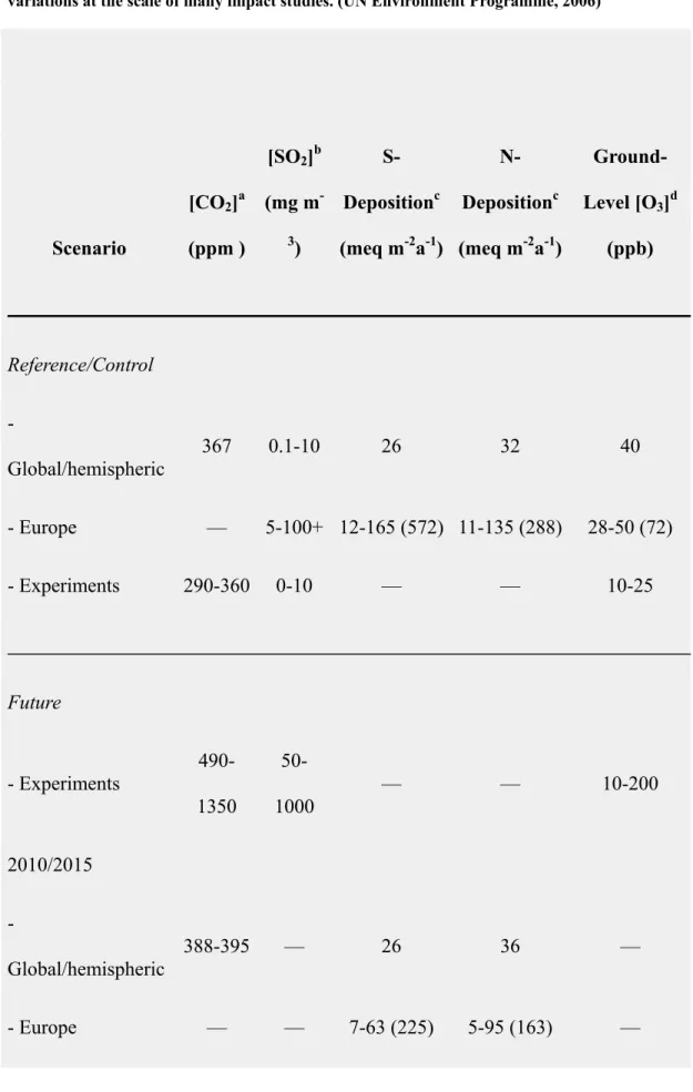
Table 8.1 : Some illustrative estimates of reference and future levels of atmospheric constituents that typically are applied in model-based and experimental impact studies. Global values are presented, where available. European values also are shown to illustrate regional variations at the scale of many impact studies. (UN Environment Programme, 2006)
Scenario [CO2]a (ppm ) [SO2]b (mg m -3) S-Depositionc (meq m-2a-1) N-Depositionc (meq m-2a-1) Ground-Level [O3]d (ppb) Reference/Control - Global/hemispheric 367 0.1-10 26 32 40 - Europe — 5-100+ 12-165 (572) 11-135 (288) 28-50 (72) - Experiments 290-360 0-10 — — 10-25 Future - Experiments 490-1350 50-1000 — — 10-200 2010/2015 - Global/hemispheric 388-395 — 26 36 — - Europe — — 7-63 (225) 5-95 (163) —
39 2050/2060 - Global/hemispheric 463-623 — — — ~60 - Europe — — 8-80 (280) 5-83 (205) — 2100 - Global/hemispheric 478-1099 — — — >70 - Europe — — 6-49 (276) 4-60 (161) —
a Carbon dioxide concentration. Reference: Observed 1999 value
Experiments: Typical ranges used in enrichment experiments on agricultural crops. Some controls used ambient levels; most experiments for future conditions used levels between 600 and 1000 ppm (Strain and Cure, 1985; Wheeler et al., 1996). Future: Values for 2010, 2050, and 2100 are for the range of emissions from 35 SRES scenarios, using a simple model; note that these ranges differ from those presented by TAR WGI .
b Sulphur dioxide concentration. Reference: Global values are background levels
(Rovinsky and Yegerov, 1986; Ryaboshapko et al., 1998); European values are annual means at sites in western Europe during the early 1980s (Saunders, 1985). Experiments: Typical purified or ambient (control) and elevated (future) concentrations for assessing long-term SO2 effects on plants (Kropff, 1989).
40
deposition over land areas in 1992, based on the STOCHEM model (Collins et al., 1997; Bouwman and van Vuuren, 1999); European values are based on EMEP model results (EMEP, 1998) and show 5th and 95th percentiles of grid box (150 km) values for 1990 emissions, assuming 10-year average meteorology (maximum in parentheses). Future: Global values for 2015 are from the STOCHEM model, assuming current reduction policies; European values are based on EMEP results for 2010, assuming a "current legislation" scenario under the Convention on Long-Range Transboundary Air Pollution (UN/ECE, 1998) and, for 2050 and 2100, assuming a modification of the preliminary SRES B1marker emissions scenario
d Ground-level ozone concentration. Reference: Global/hemispheric values are
model estimates for industrialized continents of the northern hemisphere, assuming 2000 emissions; European values are based on EMEP model results (Simpson et al., 1997) and show 5th and 95th percentiles of mean monthly grid box (150 km) ground-level values for May-July during 1992-1996 (maximum in parentheses). Experiments: Typical range of purified or seasonal background values (control) and daily or subdaily concentrations (future) for assessing O3 effects on agricultural crops (Unsworth and Hogsett, 1996; Krupa and Jäger, 1996). Future: Model estimates for 2060 and 2100 assuming the A1FI and A2 illustrative SRES emissions scenarios.
41
8.2 Environmental Scenarios
8.2.1 CO2 Scenarios8.2.1.1 Reference Conditions
Aside from its dominant role as a greenhouse gas, atmospheric CO2 also has an
important direct effect on many organisms, stimulating photosynthetic productivity and affecting water-use efficiency in many terrestrial plants. In 1999, the concentration of CO2 in the surface layer of the atmosphere (denoted as [CO2]) was
about 367 ppm (see Table 8-1), compared with a concentration of approximately 280 ppm in preindustrial times. CO2 is well mixed in the atmosphere, and, although
concentrations vary somewhat by region and season (related to seasonal uptake by vegetation), projections of global mean annual concentrations usually suffice for most impact applications. Reference levels of [CO2] between 300 and 360 ppm have
been widely adopted in CO2-enrichment experiments (Cure and Acock, 1986;
Poorter, 1993; see Table 8-1) and in model-based impact studies. [CO2] has
increased rapidly during the 20th century, and plant growth response could be significant for responsive plants, although the evidence for this from long-term observations of plants is unclear because of the confounding effects of other factors such as nitrogen deposition and soil fertility changes (Joan A.Kleypas et al., Science, 1999).
8.2.1.2 Development and Application of CO
2Scenarios
Projections of [CO2] are obtained in two stages: first, the rate of emissions from
different sources is evaluated; second, concentrations are evaluated from projected emissions and sequestration of carbon. Because CO2 is a major greenhouse gas, CO2