Probabilistic properties of bit-search type compression algorithms and the backtracking attack

(1)

T.C.

PROBABILISTIC PROPERTIES OF BIT-SEARCH

TYPE

COMPRESSION ALGORITHMS

AND

THE BACKTRACKING ATTACK

(2)

T.C.

INSTITUTE OF SCIENCE COMPUTER ENGINEERING

PROBABILISTIC PROPERTIES OF BIT-SEARCH

TYPE

COMPRESSION ALGORITHMS

AND

THE BACKTRACKING ATTACK

MS Thesis

Supervisor: PROF. DR. YALÇIN

(3)

Co-T.C.

INSTITUTE OF SCIENCE COMPUTER ENGINEERING

Name of the thesis: Probabilistic Properties of Bit Search Type Compression Algorithms and the Backtracking Attack

Name/Last Name of the Student: Date of Thesis Defense:12/09/2007

The thesis has been approved by the Institute of Science.

Director

I certify that this thesis meets all the requirements as a thesis for the degree of Master of Science.

Asst. Prof. Dr. Adem KARAHOCA Program Coordinator

This is to certify that we have read this thesis and that we find it fully adequate in scope, quality and content, as a thesis for the degree of Master of Science.

Examining Comittee Members Signature

_____________________

Prof. Dr. Emin ANARIM _____________________

Prof. Dr. Ali GÜNGÖR _____________________

Prof. Dr. Nizamettin AYDIN _____________________

(4)

ABSTRACT

PROBABILISTIC PROPERTIES OF BIT-SEARCH TYPE COMPRESSION ALGORITHMS

AND

THE BACKTRACKING ATTACK

M.S. Department of Computer Engineering

Co-Supervisor: Prof. Dr. Emin ANARIM

September, 2007, 60 pages

Linear Feedback Shift Registers (LFSRs) are the pseudorandom number generators that are used as keystream generators in Stream Ciphers. LFSRs are algebraically weak systems that have some vulnerability. To overcome this weakness of LFSRs, lots of nonlinear structures are used. In this thesis, we will deal with the most common technique to use nonlinearity in stream ciphers, which is called the compression algorithms. We investigate the probabilistic properties of the most common ones of these compression algorithms. They are SSG, BSG, ABSG, MBSG and EBSG. We also proposed a new attack to the EBSG algorithms that is called the backtracking attack.

Keywords: Bit Search Generator, Pseudo-Random Sequence, Backtracking Attack,

(5)

ÖZET

NIN OLASILIKSAL OZELLIKLERI VE ümü Eylül 2007, 60 sayfa (LFSR) Anahtar Kelimeler:

(6)

ACKNOWLEDGMENTS

This thesis is dedicated to my family and my girl friend for their patience and understanding during my master’s study and the writing of this thesis.

I would like to express my gratitude to Prof. Dr. Emin ANARIM and Prof Dr. , for not only being such great supervisors but also encouraging and challenging me throughout my academic program.

I wish to thank ,

Asst. Prof. Dr. H. Asst. Prof. Dr. M. K

for their help on various topics in the areas of probability and cryptology, for their advice and time.

(7)

LIST OF FIGURES

FIGURE 1: THE BASIC BLOCK CIPHER………...5

FIGURE 2: BASIC STREAM CIPHER……….5

FIGURE 3: THE LINEAR FEEDBACK SHIFT REGISTER………..10

FIGURE 4: NONLINEAR COMBINATION GENERATOR………..13

FIGURE 5: NONLINEAR FILTER GENERATOR……….14

FIGURE 6: ALTERNATIVE STEP GENERATOR……….14

FIGURE 7: SHRINKING GENERATOR……….15

FIGURE 8: BLOCK DIAGRAM REPRESENTATION OF BSG AND ABSG………..31

FIGURE 9: ANOTHER DEFINITION OF THE MBSG ALGORITHM……….34

FIGURE 10: STM FOR PROBABILITIES OF MEMORY BITS………...40

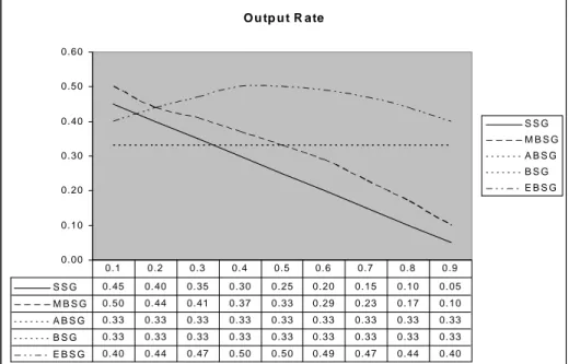
FIGURE 11: VARIATION OF THE OUTPUT RATES OF COMPRESSION ALGORITHMS…....41

FIGURE 12: DISTRIBUTION OF ZEROS IN THE OUTPUT SEQUENCE……….42

(10)

LIST OF SYMBOLS / ABBREVIATIONS

⊕ : XOR, Exclusive or, modulo 2 addition

LFSR: Linear Feedback Shift Register

IID: Independent Identically Distributed

PRNG: Pseudo Random Number Generator

SSG: Self Shrinking Generator

BSG: Bit Search Generator

MBSG: Modified Bit Search Generator

EBSG: Editing Bit Search Generator

ANF: Algebraic Normal Form

SG: Shrinking Generator

s : Input Sequence

Nn: Number of nodes at depth n

Ln: Number of leaves at depth n

Rate(C, f): Output rate of (C, f)

Podd: Probability of getting odd codeword in the first state

Peven: Probability of getting even codeword in the first state

P’odd: Probability of getting odd codeword after the first state

(11)

1. INTRODUCTION

Security is the most important concept as far as communication is concerned. Cryptography is a science that deals with hiding the content of the messages that will be transmitted one point to another. Before the modern era, people were dealing with simple cryptographic algorithms which are simple and small effects on the message such as changing the order of letters, shifting letters in the alphabet, etc. Development in technology leads people to make more secure algorithms. These algorithms are called symmetric and asymmetric encryption. During the thesis, we will deal with the key stream generation in stream ciphers which are the subset of symmetric key encryption.

The most important subject in stream ciphers is to design a system that produces random looking output sequences. Stream ciphers use pseudorandom number generators as a secret key.

Linear Feedback Shift Registers (LFSRs) are the pseudorandom number generators that they form the core like structure of most of the stream ciphers or we use them as a stream cipher. LFSRs produce random sequences with using their linear function. The resulting output sequence is a linearly dependent structure and the input sequence can be easily evaluated within a small set of algebraic operations from any subpart of the output sequence. To overcome this weakness of LFSRs, lots of nonlinear structures are used.

In this thesis, we deal with one of the most common technique to use to add nonlinearity to the stream ciphers, which is called compression algorithms. We investigate the probabilistic properties of the most common ones of these compression algorithms. They are SSG, BSG, ABSG, MBSG and EBSG. We also propose a new attack for the EBSG algorithm that is called the backtracking attack.

(12)

The outline of thesis is like that in section 2, some detailed definitions on cryptology are given and in section 3, stream ciphers are discussed, in section 4, the compression algorithms are introduced. The derivation of probabilistic properties of compression algorithms are given in section 5. The section 6 discusses the new approach for cryptanalysis of EBSG called the backtracking attack.

(13)

2. CRYPTOLOGY

Cryptology is the science that provides ways to protect and to capture the information in an online or offline transmission. It consists of two subfields called cryptography and cryptanalysis. The cryptography is deals with the protection of data, developing new algorithms, protocols, systems, etc. The cryptanalysis is a necessity of improving the cryptography; people also develop new structures, theorems, etc. to attack the cryptographic system.

2.1 CRYPTOGRAPHY:

As mentioned before, cryptography is the way of protecting the information. The cryptographic systems are mostly related with four basic security services which are listed below in Stallings (2003):

• Confidentiality: The protection of data from unauthorized disclosure.

• Data Integrity: The assurance that data received are exactly as sent by an

authorized entity.

• Authentication: The assurance that the communicating entity is the one that it

claims to be.

• Non-Repudiation: Provides protection against denial by one of the entities

involved in a communication data block: takes the form of determination of whether the selected fields have been modified.

The necessity of such services affects the selection of system to protect our data. Generally, besides the usage of security services the cryptographic algorithms also take an important point in our security structures. We can firstly group the cryptographic algorithms in two, the symmetric key encryption algorithms and the asymmetric key encryption.

Before defining the types of encryption algorithms, we have to define the concept, encryption. Encryption is a way to hide the content of the data with using set of rules and a secret key. The considerations of encryption stated with lots of principle. Te

(14)

most known one is that the Kerckhoff’s Principle Stamp and Low (2007), due to this principle our encryption method is publicly known and the secret key will only be known for parties who use the secure communication line.

We have also introduced the basic terms that are used in the cryptographic encryption algorithm. These terms are:

• Secret Key is a value for which we use to alter the input message.

• Plaintext is a input message that will be encrypted using an algorithm and a secret key.

• Ciphertext is a resulting value which is encrypted by an encryption algorithm and using the secret key.

There are also methods that do not need any secret key for producing a secret contented output (ciphertext), for example, the hash functions Stallings (2003), which we will not introduce it in our study.

Symmetric key encryption systems are divided into two groups, called as block and stream ciphers. The most important property of the symmetric key encryption is that the same key is used for both encryption and decryption.

The term asymmetric key encryption is generally known as public key encryption Goldreich (2001). Comparing with the symmetric key encryption techniques, the asymmetric encryption systems use different keys for encryption and the decryption. On the other hand, as mentioned in Stallings (2003), the number theory plays an important role in public key encryption. We generally use asymmetric key encryption for key distribution systems.

As mentioned above the symmetric key encryption techniques can be classified into two groups, the block ciphers and the stream ciphers.

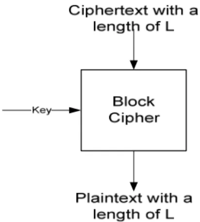
Block ciphers is a system that takes L-bit input and produces L-bit output with using a variable length (key length is up to the specifications of algorithm) secret key. Block by block encryption is realized in Block Ciphers that is why we call them block

(15)

ciphers. The most important property of block cipher is the Feistel Network Stallings (2003), which was built by Horst Feistel. This structure is used for mostly all modern block cipher algorithms.

Stallings, W., 2003. Cryptogrphy and the Network Security. New Jersey : Prentice Hall, 3rd Edition

Figure 1: The Basic Block Cipher

The most common block cipher algorithms are DES (Data Encryption Standard) Mao (2003) and AES (Advanced Encryption Standard) Stallings (2003).

Stream ciphers (Menezes at al. 1997), Stamp and Low (2007) are another important class of symmetric key encryption systems which use bit by bit encryption instead of block by block encryption. In block ciphers, we use an algorithm that provides diffusion and collusion like properties to the ciphertext. But in stream cipher the most important think is the producing a pseudo-random keystream from secret key. The encryption operation is realized with a simple XOR operation. The basic structure of the stream ciphers can be summarized as in the following figure.

Seren, Ü., 2007. Analysis of Compression Techniques and Memory Bit Efffects on Compression for Pseudo-Random Generation

Engineering Department.

(16)

Stream ciphers are more suitable for fast implementation in hardware implementation than block ciphers.

2.2 CRYPTANALYSIS

As mentioned before, cryptanalysis is the way to improve the cryptographic systems. In other words, cryptanalysis is a study for breaking the cipher. In general, we use the “cryptanalytic attack” for the operation of studying all of the properties of the system and finding weaknesses as a result of that to breaking the cipher. According to the Stallings (2003), cryptanalytic attacks rely on the nature of the algorithm plus perhaps some knowledge of the general characteristics of the plaintext or even some sample plaintext-ciphertext pairs. This type of attack exploits the characteristics of the algorithm to attempt to deduce a specific plaintext or to deduce the key being used. If the attack succeeds in deducing the key, the effect is catastrophic: All future and past messages encrypted with that key are compromised.

The most common cryptanalysis technique is the brute force attack, which is also known as exhaustive key search, is the upper bound for the complexity of breaking the cipher. This attack tries all the possible keys in the algorithm to get the correct one. The cryptanalyst, who wants to make his attack more efficient than exhaustive search, has to decrease search space of his cryptanalysis algorithm.

We know that the upper bound for the complexity of an attack is the complexity of the brute force attack for every algorithm. So our purpose has to decrease the number of possibilities to make the cryptanalysis more efficient. Cryptographic algorithms consist of linear and non-linear structures. These structures always improve the security of the algorithm but sometimes they can be the weakest part of the system. The cryptanalysis of the algorithm is a complicated work that the analysis of the system that we consider the length of the ciphertext, plaintext and the secret key and algebraic, statistical, etc. like properties of the algorithm to break the cipher.

According to the Stallings (2003), the most common types of cryptanalytic attacks and their properties for the Kerckhoff’s Principle are listed below:

(17)

• Ciphertext Only Attack: The knowledge of the encryption algorithm and the ciphertext to be decoded is enough to break the cipher

• Known Plaintext Attack: We have to know the encryption algorithm, ciphertext to be decoded and one or more ciphertext-plaintext pair that are formed with the secret key.

• Chosen Plaintext Attack: The encryption algorithm, ciphertext to be decoded and plaintext message chosen by the cryptanalyst, together with its corresponding ciphertext generated with the secret key are required.

• Chosen Ciphertext Attack: The encryption algorithm, ciphertext to be decoded and purported ciphertext chosen by the cryptanalyst, together with its corresponding decrypted plaintext generated with the secret key are necessary to crack the algorithm.

• Chosen Text Attack: The encryption algorithm, ciphertext to be decoded, plaintext message chosen by the cryptanalyst, together with its corresponding ciphertext generated with the secret key and the purported ciphertext chosen by cryptanalyst, together with its corresponding decrypted plaintext generated with the secret key.

(18)

3. STREAM CIPHERS

As mentioned before stream ciphers are kind of symmetric encryption algorithms that they operate on the plaintext bit by bit to produce the ciphertext. Stream ciphers can be classified into three groups: the one time pad, the synchronous stream ciphers and the self-synchronous stream ciphers to the (Menezes et al. 1997).

In some resources, one time pad cannot be accepted as a stream cipher. The one time pad means that we have a system that encrypts the plaintext using a key that has the same length with plaintext and also the length of resulting ciphertext will be the same as the secret key. The most known example for one time pad type stream ciphers the Vernam Cipher, see (Menezes at al. 1997). While a one-time pad cipher is provably secure (provided it is used correctly), it is generally impractical since the key is the same length as the message.

According to the definition in (Menezes at al. 1997), a synchronous stream cipher is one in which the keystream is generated independently of the plaintext message and of the ciphertext. Properties of synchronous stream cipher are defined below.

• In a synchronous stream cipher, both the sender and receiver must be synchronized using the same key and operating at the same position within that key – to allow for proper decryption. If synchronization is lost due to ciphertext digits being inserted or deleted during transmission, then decryption fails and can only be restored through additional techniques for re-synchronization. Techniques for re-synchronization include re-initialization, placing special markers at regular intervals in the ciphertext, or, if the plaintext contains enough redundancy, trying all possible keystream offsets.

• A ciphertext digit that is modified (but not deleted) during transmission does not affect the decryption of other ciphertext digits.

• As a consequence of the first property, the insertion, deletion, or replay of ciphertext digits by an active adversary causes immediate loss of synchronization,

(19)

and hence might possibly be detected by the attacker. As a consequence of the second property, an active adversary might possibly be able to make changes to selected ciphertext digits, and know exactly what affect these changes have on the plaintext. This illustrates that additional mechanisms must be employed in order to provide data origin authentication and data integrity guarantees.

There are two more structures that are really an important issue in stream ciphers called the Linear Feedback Shift Registers (LFSRs) and the Boolean Functions.

3.1 LINEAR FEEDBACK SHIFT REGISTERS (LFSRs)

In (Menezes et al. 1997), Linear Feedback Shift Registers are used in many of the keystream generators that have been proposed in the literature. The key point that makes LFSRs important in stream cipher design is that they can produce random looking numbers to the given key value.

There are several reasons that make LFSRs important:

• LFSRs are well-suited to hardware implementation • They can produce sequences of large periods

• They can produce sequences with good statistical properties

• Because of their structure, they can be readily analyzed using algebraic techniques.

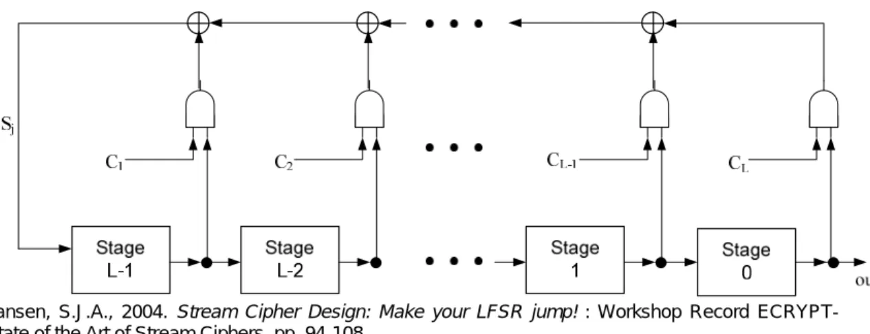
To sum up, we use LFSRs for achieving the requirements in the former section. The following figure defines the working principle of the LFSR with a length of L, each Ci represent the feedback coefficient, the closed semi-circles shows the logical

AND gates, and the feedback bit Sj is the modulo 2 sum of the contents of those

(20)

Jansen, S.J.A., 2004. Stream Cipher Design: Make your LFSR jump! : Workshop Record ECRYPT-State of the Art of Stream Ciphers, pp. 94-108

Figure 3: The Linear Feedback Shift Register

Definition 2.1: Figure 2.1 denotes polynomial F(D) = 1+C1D+C2D2+…+CLDL. This

polynomial is called connection polynomial which is also called the feedback polynomial Jansen (2004, pp. 94-108). and defined as

F (D):=

∑

= L i i iD C 0 (1)

The degree of the connection polynomial is equal to the length of the LFSR.

Definition 2.2: Assume that, we have an LFSR with a length of L, the Lth order

recursion is commonly represented by its Characteristic Polynomial, C(D), also of degree L Jansen (2004, pp. 94-108), as shown in below:

C (D):=

∑

= − L i i L iD C 0 (2)

Definition 2.3: The functions F and C are reciprocal of each other. That means, this

relation is expressed as C(D) = DLF(D-1) Jansen (2004, pp. 94-108).

Another way to look at the LFSR is to consider it as a Linear Finite State Machine as in Jansen (2004, pp. 94-108). In this case the state of the LFSM is represented by a vector σ = (t σ ,_{n 1}t₋ σ_{n 2}t₋ , …, σ ), where ₀t σ denotes the content of memory cell Mi _it after t transitions. As the finite state machine is linear, transitions from one state to

(21)

the next can be described by a multiplication of the state vector with a transition matrix T, i.e. σ =t+1 σ T, for tt

T =                 − − 1 2 1 1 0 0 0 1 0 0 0 1 0 0 0 c c c c L L L K M M O M M K K K

It can be seen that the matrix is equal to the so called companion matrix of the polynomial C(D). The characteristic polynomial of T in linear algebra sense, i.e. det(DI-T), precisely equals this polynomial and, hence, C(T) = 0. So the companion matrix plays the role of a root of C and, consequently it can be used to form solutions of the recursion equation.

Definition 2.4: Assume that we have an LFSR with a period of L. If the LFSR

produce a sequence with a length of 2L-1 without any recursion, these LFSRs are called the maximum length LFSR

At last, we must be careful about the initial key value of the LFSR. Because, if we use the key with all zero will makes LFSR to produce a sequence of all zero.

3.2 BOOLEAN FUNCTIONS:

Boolean functions are another important element of the stream cipher concept. They maps one or more binary input variable to one binary output.

Definition 2.5: In , Boolean functions f: F₂n F2 map binary vectors

of length n to the finite field F2.

(22)

(2006), among the classical representations of Boolean functions, the one in which is most usually used in cryptography and coding is the n-variable polynomial representation over , F2 of the form

f(x) = i i N i i j j i N i∈

⊕

Ρ( )a _∈x _= ∈

⊕

Ρ( )a x     ∏ ,

where P(N) denotes the power set of N = {1, 2, …, n}. Every coordinate xi appears in

this polynomial with exponents at most 1, because every bit in F2 equals its own

square. This representation belongs to F2 [x1, … xn]/(x ⊕x xn ⊕xn

2 1 2

1 ,K, ). This is

called the Algebraic Normal Form (ANF) Carlet (2006).

Definition 2.6: According to the ,w_H(f):=#{x∈F₂n: f(x)≠0}is the Hamming weight of a Boolean function while the Hamming distance between two such functions is ) ( )} ( ) ( : { # x F2 f x g x wH f g n ≠ = ⊕ ∈

In other words, Hamming weight is the number of ones in the vector and the Hamming distance of two functions is that the Hamming weight of modulo two-addition of these two functions.

Definition 2.7: According to the Seren (2007), functions of degree at most one are

called affine. The set of all affine functions in n variables is denoted as An. We can

write }. 0 , : {a0 a1x1 a2x2 a x a F2 i n An = + + +K+ n n i∈ ≤ ≤

And also According to the , while there are only 2n+1 (out of 22n total) affine Boolean functions, they form a significant class of functions and are extensively used in applications.

Continuing from Seren (2007), High nonlinearity for Boolean function is desired objective because it decreases the correlation between the output and the input

(23)

variables or a linear combination of input variables many of the attacks against stream ciphers succeed with the help of weakness of such a correlation between the combining Boolean function and some affine function.

Definition 2.9: According to the Seren (2007), let X₁,X₂,K,X_n be independent random variables, each taking the values 0 and 1 with probability 1/2. A Boolean function f(x1,x2,K,xn) is said to be t-th order correlation immune, if for each subset of t variables X₁,X₂,K,X_n with1≤i₁ ≤i₂ ≤K≤i_t ≤n, the random variable Z = f(X₁,X₂,K,X_n)is statistically independent of the random vector X.

3.3 TYPES OF STREAM CIPHERS

Generally, stream ciphers are divided into three groups, in (Menezes et al. 1997): • Nonlinear Combination Generators

• Nonlinear Filtering Generators • Clock-Controlled Generators

Continuing from (Menezes et al. 1997), one general technique for destroying the linearity inherent in LFSRs is to use several LFSRs in parallel. The keystream is generated as a nonlinear function f of the outputs of the component LFSRs; this construction is illustrated in the following figure. Such keystream generators are called nonlinear combination generators, and f is called the combining function.

(24)

Definition 2.10: According to the (Menezes et al. 1997), the definition of a nonlinear

combination generator is like that a product of m distinct variables is called an mth order product of the variables. Every Boolean function f (x1, x2, …, xn) can be written

as a modulo 2 addition of distinct mth order products of its variables, 0

expression is called the algebraic normal form of f. the nonlinear order of is the maximum of the order of the terms appearing in its algebraic normal form.

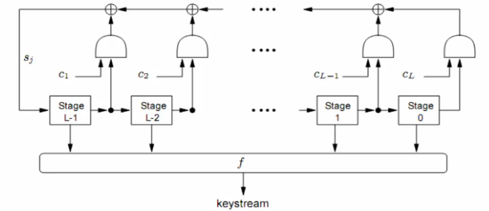
According to the Seren (2007), the nonlinear filter generator has different design principle. There is one LFSR and its different elements are used as an input of the Boolean function. There is an example for the nonlinear filter generator in the following figure

Figure 5: Nonlinear Filter Generator

The clock-controlled generators can be expressed into two groups. The first one is the alternating step generator. In this type of clock-controlled generator one LFSR is used to clock the other two LFSRs as shown in the following figure.

(25)

We can summarize the operation of alternating step generator, as in (Menezes et al. 1997), as follows:

1. Register R1 is clocked. 2. If the output of R1 is 1 then:

R2 is clocked; R3 is not clocked but its previous output bit is repeated.

(For the first clock cycle, the “previous output bit” of R3 is taken to be 0.) 3. If the output of R1 is 0 then:

R3 is clocked; R2 is not clocked but its previous output bit is repeated.

(For the first clock cycle, the “previous output bit” of R is taken to be 0.)

4. The output bits of R2and R3 are XORed; the resulting bit is part of the keystream.

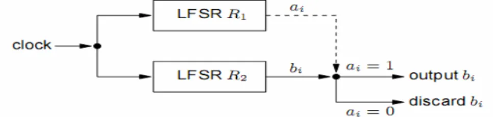
Second type of clock-controlled generators are that the Shrinking Generator. The working principle of the Shrinking generator is as followsn summarize the operations of this generator in the following three steps (Menezes et al. 1997):

1. Registers R1 and R2 are clocked.

2. If the output of R1 is 1, the output bit of R2 forms part of the keystream. 3. If the output of R1 is 0, the output bit of R2 is discarded.

Figure 7: Shrinking Generator

3.4 SECURITY OF STREAM CIPHERS

As far as the cryptanalysis of a stream cipher concerned the following concepts are playing an important role to attack the system Seren (2007):

(26)

• Time Complexity: Can be defined as required number of operations needs to be processed to apply attack and to reach success.

• Data Complexity: It can be defined as the required amount of keystream material which is needed to guarantee the success of attack.

• Memory Complexity: It can be defined as the required memory to attack the cipher. It is just like a combination of both the time and data complexity.

The list of the important cryptanalysis methods are listed below

Trade-off Attacks: These types of attacks are generally related with two of the three

concepts that we have declared above, time, data and memory complexity. The main purpose of the trade-off attacks is to decrease the search complexity of the exhaustive search into data and time complexity, see Babbage (2006) for detailed information.

Algebraic Attacks: These types of attacks try to find a linear equation with a higher

degree between input and output of the stream cipher. Then, using some techniques that are declared in Shamir and Kipnis (1999), Courtois and Patarin (2003) and Armknecht (2006), try to solve this multivariate equations.

Distinguishing Attacks: distinguishes a stream of bits from a perfectly random

stream of bits, that is, a stream of bits that has been chosen according to the uniform distribution. See Johansson and Jönsson (1999) for more information.

Correlation Attacks: According To Seren (2007) and Johansson and Jönsson (1999),

in the correlation attack, attacker aims to find a correlation between input variables to the combining function and the output from the combining function, and then use this correlation to obtain information about the correlated input variables.

(27)

4. COMPRESSION ALGORITHMS

Generally, we use compression algorithms to compress the data to make them portable. And also the resulting compressed data must be as small as possible and this small amount of data have to contain much of data from the original one. It is more different, when we think about compression in cryptographic manner. The cryptographic compression algorithms have to contain least data in a maximum size that it can hide from the original one.

The cryptographic compression algorithms are especially used to add nonlinearity to the pseudo-random sequences. As we mentioned that pseudo-random sequences has weaknesses to the Algebraic attacks that you can find more information about them in Shamir and Kipnis (1999), Courtois and Patarin (2003) and Armknecht (2006).

We can use compression function while compressing the output of the LFSR like pseudo-random number generator. The compression function takes n bits of input and produces m bits of output, where n

can be classified to the value of output rate.

Decimation based compression algorithms are good example for cryptographic compression algorithms. These are used as a second structure to compress the output of the PRNG structure. The most common decimation algorithms are SSG, BSG, ABSG, MBSG and EBSG.

4.1 A COMPRESSION MODEL FOR PSEUDO-RANDOM GENERATION

As we mentioned before our purpose is to decrease the vulnerabilities of a pseudo-random generator. To make the keystream more secure, we will use some compression algorithms. These compression algorithms delete or insert bits to the original sequence to prevent the keystream from attacks that are related with the algebraic or correlation type properties of pseudo-random outputs.

(28)

each word w is a prefix of a random input sequence with probability 1/2|w|, and all words are assumed to be independent.

4.1.1 Prefix Codes and Binary Trees

The definition in Gouget and Sibert (2006, pp. 129-146) is that a binary code is a subset of words of {0, 1}+. The language C* of a binary code C is the set of all binary words that are concatenation of words in C. a code C is a prefix code if no codeword has a strict prefix in C. Notice that, in this case, the words of C* parse into codewords in a unique manner. A code is a maximal prefix, when no other prefix code contains it. A code C is right complete if every word w can be completed into a word v=ww'

in C.

According to proposition 3.1 in the Gouget and Sibert (2006, pp. 129-146), a code is maximal prefix if, and only if, it is prefix and right complete

Proof. Suppose C is maximal prefix. Let w be a non-empty word which has no prefix

in c. As c is maximal prefix, C∪{w}is not a prefix code, so w has a right multiple in C. Hence, C is right complete. Conversely, let C be prefix and right complete, and C’ be a prefix code that contains C. Letw∈ . As C is right complete, w has a rightC

multiple w ’ in C*. Let them be the smallest prefix of w ’ in C. As C is prefix, this implies m = w, so we havew∈ , and consequently C C'=C.Therefore, C is maximal prefix.

4.1.2 General Framework

We have an infinite input sequence of bits s=(si)i≥0,a binary prefix code C and a

mapping f :C →{0,1}* called the compression function Gouget and Sibert (2006, pp. 129-146). We call f(C) the output set. The sequence consist of sequence of codewords w=(wi)i≥0, each w being the unique codeword such thati w K0 wi is a

prefix of s that belongs to C*. Each w is the n mapped by f to its image in f(C). The output sequence is (f(w_i))_i_≥₀ , seen as a bit sequence. We denote this output sequence by

(29)

) ( ,f s C Enc y=

Definition 3.1: The output rate of the pair (C,f), denoted by Rate(C,f), is the average

number of output bits generated by one bit of a random input sequence Gouget and Sibert (2006, pp. 129-146).

However, some exceptional cases hold in this situation. For example, we cannot get an output 1 from an input sequence, C = {00}. Continuing from the Gouget and Sibert (2006, pp. 129-146), In order to apply the framework to every possible input sequence, it is then necessary to determine what the requirements on the following components are:

• The choice of C must enable the parsing of every random input sequence,

• The choice of f must be such that, for uniformly distributed input sequences, the corresponding output sequences also follow the uniform distribution.

4.2 REQUIREMENTS ON C

First, there are some straight requirements on C. Only the prefix codes are considered in the framework that is expressed in Gouget and Sibert (2006, pp. 129-146). Indeed, if C contained two distinct words w and w ’ with w a prefix of w ’, then w would never appear in the decomposition w of s. Therefore, we may delete from C all the codewords that already have a prefix in C without loss of generality, thus transforming C into a binary prefix code. Next, we want every random input sequence to be processable. This implies that C is right complete. Overall, in order to effectively process any random input, we introduce the following definition:

Definition 3.2: A binary code C is suitable if it is prefix and if the expected length

E(C) of an element of C in the decomposition of a random input sequence is finite.

As mentioned in proposition 3.2 in the Gouget and Sibert (2006, pp. 129-146): For a suitable code C, the following equality holds:

1

(30)

Proof. A binary tree corresponds to C.L and _n N are denoted as the number of _n

leaves and nodes of depth n. If we have L0 =0,then we will have N0 =1,

and where n L +_n N =_n 2N_n₋₁.

∑

≤ ≤ = n k n n n L S 0 2 (1) n n L 2 = 1 1 2 − − n n N -N_nn 2 (2) n n n n n N N N S 2 1 2 0 − = − = (3)

The proof of N_n =O(2n) will be enough. Now, Nn is the number of nodes of depth

n, and a random input sequence begins with n bits corresponding to such a node with probabilityN_nn

2 . For each one of these nodes, the first word of the input sequence recognized as a word of C has length at least n. Thus, these nodes contribute at least nN_nn

2 to E(C). As E(C) is finite, this implies that tends to 0 when n tends to ∞ .

Therefore, in the case of a suitable code, E(C) is equal to the mean length of the words of C for the uniform distribution on the alphabet {0, 1}. So, according to the proposition 3.3 in the Gouget and Sibert (2006, pp. 129-146), C be a suitable code. Then, the equality is as follows:

∑

∈ = c w w w C E | | 2 | | ) ( 4.3 REQUIREMENTS OF f

When we look at the requirements on f(C), f(C) can be any set of words including ε (the empty word). Furthermore, there will be at least two more non-empty words. One of them will star with 1 and the other is 0. It is possible to make random looking

(31)

output for random inputs. Moreover, it must be possible to construct every binary sequence with the elements of f(C).

In order to be able to process every random input sequence, we introduce the following definition, which corresponds to the requirement of Definition 3.2:

Definition 3.3: Assume that C is suitable and f be the compression function with the

definition: f :C→{0,1}*. We can easily say that the pair (C,f) is a proper encoder if the expected length E(f(C)) of the image by f of an element of C in the decomposition of a randomly chosen input sequence is finite and nonzero, Gouget and Sibert (2006, pp. 129-146).

The Proposition 3.4 in Gouget and Sibert (2006, pp. 129-146) says that for a proper encoder (C, f), the expected length of the image by f of an element of C in the decomposition of a randomly chosen input sequence, denoted by E (f(C)), is given by

∑ ∈ = c w w w f C f E | | 2 | ) ( | )) ( (

Definitions 3.2 and 3.3 ensure the finiteness of E(C) and E(f(C)), so according to the proposition 3.5 in Gouget and Sibert (2006, pp. 129-146), the output rate of a proper encoder (C, f) is given by ) ( )) ( ( ) , ( C E C f E f C Rate =

The randomness properties and the equality in number of 1s and 0s in the output sequence are provided by the distribution of output sequences. Therefore, we need, for every n 1: ∑ = ≥ ∈ ,| ( )| , ( ) 0 | | 2 1 n w f n w f C w w = ∑ = ≥ ∈ ,| ( )| , ( ) 1 | | 2 1 n w f n w f C w w

(32)

4.3.1 The Prefix Code Output Case

First of all, considering the case where f(C) is a prefix code. If it contains two elements, the only possible choice such that the probability distribution of the output for random inputs is that of a random sequence is f(C) = {0,1}. In this case, 0 and 1 must have probability 1/2 to appear in the output sequence for a random input sequence Gouget and Sibert (2006, pp. 129-146).

If there are more than 2 elements for f(C), then, given a random input sequence, knowing the output sequence, we can retrieve more information on the first element of C than in the case f(C) = {0,1}.

According to the proposition 3.6 in Gouget and Sibert (2006, pp. 129-146) again, Let (C, f) be a proper encoder, and, for x∈ f(C), let

∑

− ∈ = 12| | 1 ) ( f w w x P . Then, for a

random input sequence s, each word of the decomposition of s over C has average length E(C), and it is known with average entropy.

∑

∈ + ) ( ) ( log ) ( ) ( C f x x P x P C E

Proof. For x ∈f(C), let us denote by C the preimage of x in C. Then, the probability _x

that the first element of C recognized in a random input sequence is

∑

∈ = x C w w x P _| _| 2 1 ) ( .

Similarly, the expected length of an element in the preimage of x is E(Cx) =

∑

∈ xC w w w x P | | 2 | | ) ( 1

. At least we compute the entropy on the elements Cx in:

∑

∈ ∈ =− + − = x C w x C w w x P x P x P x P C H x _x _x _x log( ( ) | |) 2 ) ( 1 2 ) ( 1 log 2 ) ( 1 ) ( _|_| _| _| _|_| ) ( log ) ( 2 1 ) ( ) ( log 2 | | ) ( 1 | | | | E C P x x P x P w x P x C w x C w x w w + = + =

∑

∈ ∈

(33)

The average number of bits retrieved is therefore

∑

_∈

)

(C ( ) ( )

f

x P x E Cx = E(C) for a

random input sequence, so it does not depend on f(C). The average entropy is

∑

∈ ∈ ( ) + = + ( ) ) ( log ) ( ) ( )) ( log ) ( )( ( c f x c f x x P x P C E x P C E x P _x , , with

∑

∈ ( ) = 1 ) ( log ) ( c f x x P x P .

It is usually possible that the given a suitable code C, to divide C into two equiprobable subsets (the probabilities of leaves in the tree being of the form _n

2 1 with n

mapping f :C →{0,1} such that 0 and 1 are output with probability 1/2.

Therefore, in order to maximize the entropy for a given suitable code C, the value of |

∑

∈ ( ) ) ( log ) ( c f x x P x

P | should be as small as possible, which implies # (f(x)) = 2.

Therefore the optimal set is f(C) = {0, 1}, with 0 and 1 having the probability 1/2 to be output for a random input sequence, Gouget and Sibert (2006, pp. 129-146)

4.3.2 The Non-prefix Output Case

Consider the cases there are no in f(C), but also f(C) is not a prefix code. Let C(y) be the set of words of C such that, for everyw∈C( y), the sequence y begins with w. Then, the probability that s begins with w is up to y.

General Case. We now suppose that ε can belong to the output set f(C).

According to the proposition 3.7 in Gouget and Sibert (2006, pp. 129-146), Let (C, f) be a proper encoder such that f(C) containsε . Then, there exist a proper encoder (C’,

f’) such that f(C’) does not contain ε and that, for every infinite binary sequence s,

that is ). ( ) ( ,' ' , s Enc s EncC f = C f

(34)

Moreover, defining

∑

− ∈ = ) ( 1 2| | 1 ε ε f w w P , so, ) ( 1 1 ) ' ( E C P C E ε − = and ( ( )). 1 1 )) ' ( ' ( E f C P C f E ε − =

Proof. Denote by C the set of preimages of_ε ε , and by C the complement of _ε C in _ε

C. Let C’ be the binary code defined byC'=C_ε*C_ε , that is, the set of binary words that parse into a sequence of words ofC , followed by a word of _ε C_ε. Consider the function f’ that maps each element ww’ of C’, withw∈C_ε*, andw'∈C_ε, to f(w’). As the decomposition is unique, f’ is well-defined. Moreover, for every input sequence s, the equality Enc_C_,_f(s)=Enc_C_,'_f_'(s)is obvious satisfied. In the end,

) ( ) '

(C f C

f = \{ε }, so the image of f’ does not contain ε .

There remains to show that the new pair (C’, f’) is also a proper encoder. First, C’ is also a prefix code because of ubiquity of the decomposition over C.

Next, as the length of ε is 0, we have

ε ε ε ε ε P C f E w f w f C f E C v C w C v n v C w n v w v  × = −       = =

∑

∑ ∑

∑

∈ ∈ ∈ + ≥ ∈ 1 )) ( ( 2 | ) ( | 2 1 2 | ) ( | )) ' ( ' ( _|_| _| _| _|_| _| _| , * 0

As the two encoders (C,f) and (C’,f’ ) are equivalent, they have the same output rate, which yields the same relation between E(C ) and E(C). Hence, (C ,f) is a proper encoder.

Gouget and Sibert (2006, pp. 129-146) proposed that without loss of generality, assume that f(C) does not containε . So, the optimal choice for f(C) is f(C) = {0,1}.

(35)

4.4 TYPES OF COMPRESSION ALGORITHMS

4.4.1 The SSG Algorithm

Self-Shrinking Generator is a modified version of the shrinking generator and was firstly presented in (Zenner at al. 2001, pp. 21-35). Assume that we have a random variable X | X = {x0, x1, x2 …}, which was generated by LFSR, used as an input

sequence to the SSG. The random variable Z | Z = {z0, z1, z2…}, which was

generated from X, is accepted as output. The output rate of the Self-Shrinking Generator is 1/4. According to the definition in (Zenner at al. 2001, pp. 21-35), SSG algorithm searches the bits that have the even position, if the value of bit is 1, sets the output bit as the latter bit of the even positioned bit, else the value of even positioned bit is 0, and the algorithm gives no output. We can summarize the SSG algorithm as follows: Set i := 0, j := 0 while (true) if (x[i] j := j + 1 i := i + 2

The output rate calculation is very simple for SSG algorithm. Assume that we have an evenly distributed input sequence, the occurrence of 1 in even position is 1/2 and also we know that the algorithm gives one output bit to the given two input bits that means we have L/2 output bits, if all of the bits at the even positions are 1 with the input sequence length of a L. Under the conditions that are mentioned above, we can easily say that we have the output rate of 1/4.

Example 3.1: Let X = 11010011101001000111 be the input sequence. Then the

action of SSG on X can be described as follows:

{ 1 11 { − 01 { − 00 { 1 11 { 0 10 { 0 10 { − 01 { − 00 { − 01 { 1 11

(36)

4.4.2 The BSG Algorithm

The Bit Search Generator algorithm is a kind of cryptographic compression algorithm that takes a pseudorandom input with size of L and produces the output with a size of L/3. This algorithm was firstly proposed in Gouget and Sibert (2004, pp. 60-68). And According to the (Gouget et al. 2005) and Mitchel (2004) there are two different but equivalent ways to describe it.

The random variable X | X = {x0, x1, x2 …}, which was generated by the LFSR, is

accepted as an input to the BSG. The random variable Z | Z = {z0, z1, z2, …}, which

was constructed from X, is accepted as output. The BSG algorithm works like this, first of all the x0 from input bit is set as a search bit and then, the algorithm starts to

search the bit which has the same value with x0. Assume that we find the correct bit at

the position l, if there are no bits between xl and the search bit, then, the resulting bit

will be 0 for output, otherwise, the output bit will be 1. The searching operation can be summarized as follows, the BSG algorithm searches for the patterns

_

b bi

_

b , where

i ∈{0, 1}. If i is equal to 0, then the output will be 0, else the output will be 1. The working principles of BSG algorithm in pseudo code format is as shown in below: Set i := -1, j := -1 while(true) i := i + 1 j := j + 1 b := x[i] i := i + 1 if (x[i] = b) set z[j] := 0 else while(s[i] b) i := i + 1

The second definition of BSG algorithm called as BSGDiff. BSGDiff algorithm works

on differential sequence di = xi⊕ xi+1, i Hell and Johanssoni (2005), the action

of the BSGDiff on the input differential sequence d consist in splitting up the

(37)

every such subsequence, the output bit is the first bit of the subsequence. The pseudo code of the BSGDiff is as follows:

Set i := 0, j :=0 while (true) z[j] := d[i] if(d[i] = 1) i := i + 1 while (d[i] = 0) i := i + 1 i := i + 2 j := j + 1

action of BSG on X can be described as follows: { 1 010 { 1 1001 { 0 11 { 1 010 { 1 010 { 0 00 { 0 11 { 0 101

4.4.3 The ABSG Algorithm

The ABSG algorithm is the improved version of the BSG algorithm which was proposed in (Gouget et al. 2005). The working principle of the ABSG is most likely to the BSG algorithm except the determination of the output bits. In ABSG algorithm, the output bit is selected from the input bit, the second bit of the codeword is used as an output bit. There is no change in the searching process, we look for the codewords

_

b bi

_

b , where i

ABSG algorithm gives N-bit output to the given 3N bit input. If i is equal to zero the output bit will be

_

b , otherwise b. With using the definitions about the input and

output bits in section 3.1, we can summarize the algorithm as pseudo code below:

Set i := 0, j := 0 while(true) b := x[i] z[j] := xi+1 i := i + 1 while(x[i] = _ b ) i := i + 1 i := i + 1 j := j + 1

(38)

action of ABSG on X can be described as follows: { 1 010 { 0 1001 { 1 11 { 1 010 { 1 010 { 0 00 { 1 11 { 0 101 4.4.4 The MBSG Algorithm:

MBSG algorithm is the short form of the Modified Bit Search Generator. This algorithm was firstly introduced in (Gouget et al. 2005). MBSG has the output rate of 1/3 for evenly distributed inputs. This algorithm searches the subsequences b0i1,

where i Set i := 0, j := 0 while (true) yi := xi i := i + 1 while (xi = 0) i := i + 1 i := i + 1 j := j + 1

action of MBSG on X can be described as follows:

{ 0 01 { 0 01 { 0 001 { 1 11 { 0 01 { 0 001 { 0 0001 { 1 11 { 0 01

4.4.5 The EBSG Algorithm:

The EBSG algorithm, which is the short form of the Editing Bit – Search Generator, was firstly proposed in (Ergüler et al. 2006). This algorithm is the last version of Bit – Search type decimation algorithms that gives the output rate of ½ from N – bit input sequence.

When we consider the working principles of EBSG, it shows similarities with ABSG algorithm except the difference of inserted memory bits. This memory bits after the input sequence of EBSG algorithm and defines the start points of output bits.

(39)

Assume that, we have an input sequence X = {xi}1N, and the corresponding output

sequence Z = {zj}, and also we have memory bit t with the initial of 0. First of all, the

algorithm value searches the codeword _

b bi

_

b , where i 0 from X, if i is odd, the value of t will be , otherwise it will protect the its initial value and then t will be inserted into the sequence at the position of after the codeword. the search for new codeword starts for the inserted bit. This operation continues to the end of the input sequence.

Set i := 0, j := 0, t := 0 while (true)

z[i] := x[i+1], b = s[i] i := i +1 while (x[i] = _ b ) i := i +1, t := t s[i] := t j := j+1

action of EBSG on X can be described as follows:

{ 1 010 { 1 1 1 { 0 1 001 { 1 1 1 { 1 1 1 { 0 1 01 { 0 0 0 { 0 0 0 { 1 0 10 { 0 1 001 { 1 1 1 { 1 1 1

(40)

5. PROBABILISTIC PROPERTIES OF COMPRESSION

ALGORITHMS

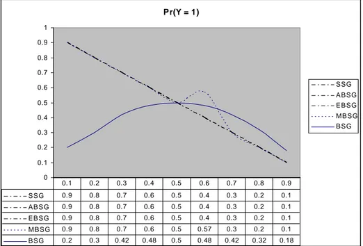
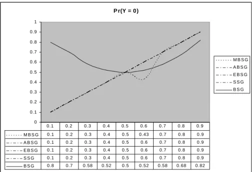
Generally, decimation algorithms compress the output of the pseudo-number generators. But it is possible that, this algorithm can be used to compress different types of data such as image, voice, etc. In this section, the output rates and output distributions of the compression algorithms (SSG, BSG, ABSG, MBSG and EBSG) are determined for the input sequence of independent identically distributed (i.i.d.) Bernoulli input with p. We found that the best result for i.i.d. Bernoulli input is 1/2 which we can say that it is also pseudo-random sequence. If we change the input distribution with respect to p, where 0.1 output rates and output distribution will be affected too. So, the system will give more information about input text than before (i.i.d. Bernoulli with 1/2). Then, we can analyze the system more easily.

5.1 BSG & ABSG:

Because of the similarities in their searching structures, in this subsection we will show the probabilistic properties of BSG and ABSG algorithms together.

First of all, we will make some general definitions, the input sequence which is called X | X = {x1, x2 ...}, is general for the entire algorithm in the paper. And the output

sequence will be the Z | Z = {z1, z2 ...}.

We will define the BSG and ABSG together, because they show nearly some operation on the input sequence. According to the Gouget and Sibert (2004, pp. 60-68), BSG algorithm searches the codeword bbib, b {0,1} and i

output bit will be 0 otherwise the output bit will be 1. In the ABSG algorithm, the output bits will be b or b for the same codewords and rules.

Situation is a bit different. According to the (Gouget et al. 2005), ABSG searches the same codeword bbib, if i = 0 the output will be b , otherwise b.

(41)

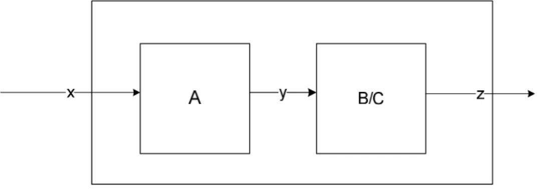
In the et al. 2007), another description of these algorithms is introduced. And

the following figure (Figure 2.1) summarizes it. For BSG we use A + B and for ABSG we use A + C to get the output.

006. A Note on the Periodicity and the Output Rate of Bit –Search Type Generators, IEEE Transactions on Information Theory (Submitted).

Figure 8: Block Diagram Representation of BSG and ABSG

Both ABSG and BSG algorithm use the “A” part of the figure above and A contains a function M (.) which produces the random variable Y | Y = {y1, y2} y to the given x. the definition of M is given the table below. The Ø symbol means that system will give an output. And the initial value of Y random variable is y0 = Ø.

Table 5.1: Mapping for BSG & ABSG

Gouget, A., Sibert, H., 2004. The Bit Search Generator. The State of the Art of Stream Ciphers: Workshop Recofrd, ss. 60-68.

We can get the following matrix from the table above

          = 1 0 1 0 1 1 1 1 0 A

And the equation

3 2 3 2 ) 1 2 ( 3 1 W I A n = + n − yi\xi-1 0 1 Ø 0 1 0 Ø 0 1 1 Ø

(42)

Continuing from Ø,

T

. And we know that P0 = (1, 0, 0)T. So,

P1 = A . P0

P2 = A . P1

…

Pn = A . Pn-1

As we know the sequence X is not evenly distributed. The probability of 0 in X is p and also 1 is 1 – p. We have

n n-1 + (1 – n-1 n n-1 + (1 – p ). n-1 n n-1 + (1 – n-1

We will get the probability vector for the first state of the Markov process is that

P1 = (0, p, 1 – p)T.

So the resulting equation is

1 2 1 2 → + → ⋅ = A P P n n → → − + = 2 ₃ ₁ 1 2 ) ) 1 2 ( 3 1 (I W P P A n n

And we will have the vector

T n n n p p P _n       ₋ ₊ ₋ ₋ ₊ ₋ = → +1 1₃(22 1), 1₃(22 1),(1 ) 1₃(22 1) 2 2n+1 2n+1, 2n+1)T

When the working principles of ABSG and BSG algorithms are concerned, they show a few dissimilarities and these are described in B and C parts of the figure 2.1. The definition of B is as follows

(43)

   ≠ = = = = φ φ φ φ 2 -i i 2 -i i y and y y and y if if Zj , 1 , 0 , where j

The algorithm C can be given as follows

   ≠ = = = = − − φ φ φ φ 2 -i i 2 -i i y and y y and y if y if y Z i i j , , 2 1 , where j

The probabilities of the Y₁N which is a Markov process of memory one with the initial conditionY₀ =φ, is as follows

) | Pr( ) | Pr( 2 1 1 1 φ φ φ φ ≠ = ≠ ≠ = = Y_i Y_i₋ Y_i Y_i₋ ) | Pr( 1= Y_i ≠φ Y_i₋₁ =φ

These probabilities are independent of the distribution of the input sequence. As we can easily see that from Table 1, whatever the p values of X is that the output rates of the BSG and the ABSG won’t change. So the result will be same as in the

al. 2007).

[

]

[ ]

N N N N H E H/N E      − + − = = 2 1 9 2 9 2 3 1

5.2 MBSG

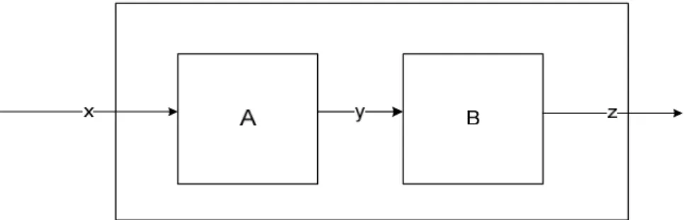
MBSG is another improved version of the BSG algorithm. As we defined before, the MBSG, which was proposed in Mitchel (2004), searches the codeword b0i1, where i b∈{0,1}. In addition to that, we can also define the MBSG algorithm as follows:

(44)

Figure 9: Another definition of the MBSG algorithm

The algorithm A contains the function M (.) which is defined in the following table

Table 5.2: Mapping for MBSG

, where y0 = Ø

The definition of the B algorithm is that Zj = yi – 1 if yi = Ø, where j

From Table 2, we will get the matrix A, which is as same as in , is shown below.           = 1 0 1 0 1 1 1 1 0 A

And we will also use the same equation

3 2 3 2 ) 1 2 ( 3 1 W I A n = + n − where,           = 1 1 1 1 1 1 1 1 1 3 W

For calculating the output distribution of MBSG we will define the probability vector . Continuing from

et al. 2007) we will get the 1 → P = (0, 1-p, 1-p). y i – 1 \ xi 0 1 Ø 0 1 0 0 Ø 1 1 Ø

(45)

To sum up, the resulting equation is that → → + →       ₊ ₋ = = 3 1 2 1 2 1 2 (2 1) 3 1 P W I P A P n n n T n n n p p p       ₋ ₋ ₋ ₊ ₋ ₋ ₊ ₋ = (2 1)) 3 2 1 )( 1 ( )), 1 2 ( 3 2 1 )( 1 ( ), 1 )( 1 2 ( 3 2 2 2 2

(

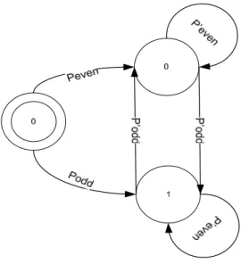
2 +1, 2 +1, 2 +1

)

= α n β n θ n

Because of the structure of the M function in MBSG the output rate will be change due to the probability distribution of input sequence. As far as the working principle of MBSG concerned we can easily see the same results as in the later subject. Because, the MBSG searches for the codeword b 0i 1, that means, MBSG looks for 1 after starting a new code to give an output. So we can say that the output probabilities are as shown in below with the initial condition y₀ =φ

1 ) | Pr( ) | Pr( 1 ) | Pr( 1 1 1 = = ≠ = ≠ ≠ − = ≠ = − − − φ φ φ φ φ φ i i i i i i y y p y y p y y

Since we are dealing with the Ø; we can define a new random variable an as in et al. 2007) to clarify the calculating output rate as in follows,

   = = . , 0 . 0 y , 1 _i otherwise if Qi we have 1 ) 1 | 0 Pr( ) 0 | 0 Pr( 1 ) 0 | 1 Pr( 1 1 1 = = = = = = − = = = − − − i i i i i i Q Q p Q Q p Q Q

Assume that we have n blocks that contribute the b 0i 1, i

have a function L(.), which gives the length of the block as in . So we have the following equation,

(46)

) 1 , ) ( Pr(L Blockn =l Qn = ) ), , 0 ( , 1 Pr(Q_n = Q_i = n<i<n+l Q_n₊_l = ) 1 , 0 , , 0 , 1 Pr( = ₁= ₁ = = = Qn₊l Qn₊l₋ K Qn₊ Qn

[

₄₄ ₄₄₄₄₃

]

4 4 2 1 4 4 4 3 4 4 4 2 1 2 ) 0 | 0 Pr( ) 0 | 1 Pr( 1₂ ₁ 1 1 − − = = ∏ ⋅ = = = − ₋ + = − − n m p i i m n i p m m Q Q Q Q 43 42 1 4 4 4 3 4 4 4 2 1 n n n n Q Q Q α ) 1 Pr( ) 1 | 0 Pr( 1 1 = = ⋅ = ⋅ ₊ n l p p ⋅ ⋅α − = −2 ) 1 (

We have found an expression for the probability of occurring a length l block, it is time to find the expected WØ (Y1N), which is created by A algorithm and independent

identically distributed Bernoulli with p. We have also two cases for this situation as in

(Al . i. Q_N =1, Pr(H =k|Q_N =1)

∑

+ < < ∀ = = = = 1 1 | 0 1 1) , , ( ) | 1) ( Pr( k i l k k i Q l Block L l Block L K

∑

+ < < ∀ − − − ⋅ − ⋅ − ⋅ ⋅ − = 1 1 | 2 2 2 2 1 ₍₁ ₎ ₍₁ ₎ ) 1 ( k i i l k L L L p p p p p p K

∑

+ < < ∀ − ⋅ − = 1 1 | 2 ) 1 ( k i i l k N p p k And we have _      − − − 1 1 k k N

ways to put k – 1 “10” pattern in N – 2 locations.

So we will have, 1 2 ) 1 ( 1 1 ₋ ₋ ⋅ − ⋅       − − − _N _k p p k k N _k

ii. QN =0, that means we will have k “10” pattern in N-1 locations so,

1 2 ) 1 ( 1 ) 0 | Pr( _⋅ − ⋅ − −      − − = = = N k p p k k N Q k H N k

(47)

When we try to calculate first and second moments to get the output rate of MBSG algorithm which is E[H/N] as in al. 2007).

[ ]

_∑

= = − ⋅ − = = = N i i N i i p Q H E 1 1 ) 1 2 ( 3 2 3 2 ) 1 Pr( ) 2 ( 3 2 ) 2 1 ( 3 2 3 2 3 2 p p p N p Np N + − ⋅ − N = + N − − N = Since,

[

]

[ ]

N p N p p N H E N H E N 3 2 3 2 3 2 3 2 / 1 + − − + = =

5.3 SSG

According to the definition of SSG, which was introduced in the former section, divides the input sequence into 2 – bit codewords, if the first bit of the codeword is zero, there will be no output; otherwise, the output will be the second bit of the codeword.

In other words, the definition of SSG is as follows; assume that the input sequence is

N i

X

X =( )₁ and resulting output sequence is Y ={y_i}₁N, which yj = x2i, if x2i – 1 =1 and

0 < j

When we consider the probabilistic properties of SSG, it normally has the output rate of ¼ that means if we have 4n – bit input, we will have n – bit output.

Claim: Pr

[

y_i =1

]

=(1− p), Pr

[

yj = 0

]

= p

Proof: Pr

[

yj =1

]

=Pr

[

x2i =1

]

=1-p, for some i > j

Claim: (Given N – bit long input)

Proof:

[

]

 

p p N i p N i M _⋅ − ⋅ −       = = ₂ ₍₁ ₎ 2 Pr , for

 

2 0≤i≤ N

Probabilistic properties of bit-search type compression algorithms and the backtracking attack

T.C.

PROBABILISTIC PROPERTIES OF BIT-SEARCH

TYPE

COMPRESSION ALGORITHMS

AND

THE BACKTRACKING ATTACK

T.C.

PROBABILISTIC PROPERTIES OF BIT-SEARCH

TYPE

COMPRESSION ALGORITHMS

AND

THE BACKTRACKING ATTACK

Supervisor: PROF. DR. YALÇIN

Co-T.C.

ABSTRACT

ÖZET

ACKNOWLEDGMENTS

TABLE OF CONTENTS

LIST OF FIGURES

LIST OF SYMBOLS / ABBREVIATIONS

1. INTRODUCTION

2. CRYPTOLOGY

3. STREAM CIPHERS

∑

∑

⊕

⊕

4. COMPRESSION ALGORITHMS

∑

∑

∑

∑

∑

∑

∑

∑

∑

∑

∑

∑

∑

∑

∑

∑

∑

∑ ∑

∑

5. PROBABILISTIC PROPERTIES OF COMPRESSION

ALGORITHMS

5.1 BSG & ABSG:

[

]

[ ]

5.2 MBSG

(

)

[

]

∑

∑

∑

[ ]

∑

∑

[

]

[ ]

5.3 SSG

[

]

[

]

[

]

[

]

[

]

 

_∑

_∑