A Locality Preserving OneSided Binary Tree
-Crossbar Switch Wiring Design Algorithm
Devrim S¸ahin
Department of Computer Science and Engineering
Bilkent University, Ankara, Turkey
[email protected]
Abstract—One-sided crossbar switches allow for a simple implementation of complete Kngraphs. However, designing these
circuits is a cumbersome process and can be automated. We present an algorithm that allows designing automatic one-sided binary tree - crossbar switches which do not exceed⌊n
2⌋ columns,
and achieves Kn graph without connecting any wires between
any three adjacent blocks, thus preserving locality in connections.
I. INTRODUCTION
One-sided switch is a special type of topology used in applications in which input terminals also serve as outputs. Instead of connecting a set of inputs X = {x1, x2, · · · , xn}
to a set of outputs Y = {y1, y2, · · · , yr}; one-sided switches
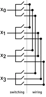
make connections from a set X onto itself. Thus, every one of the n terminals is connected to every other (n − 1), totalling to n·(n−1)2 connections. While switches in general can be represented as bipartite graphs, one-sided switches are equivalent to undirected Kn complete graphs. Figure 1 is an
example of a 4-input one-sided switch.
Fig. 1. 4-input binary tree - crossbar switch.
Since there are n = 4 inputs, each input xi should have
n − 1 = 3 ‘copies’, that is, separate routes through which xi
can connect to every other xj. In the implementation above,
this is simply achieved by making three copies of each input immediately, then making pairwise connections in the wiring part from every xi to everyxj (i 6= j).
Given the circuit above, connecting two inputs is trivial. For example, in order to establish a connection between x0
andx2, it is required and enough to close two switches (2nd
and 7th switches from above, that is, middle x
0 switch and
top x2 switch). However, each of the terminals have a fanout
of n − 1, which is not a desirable property.
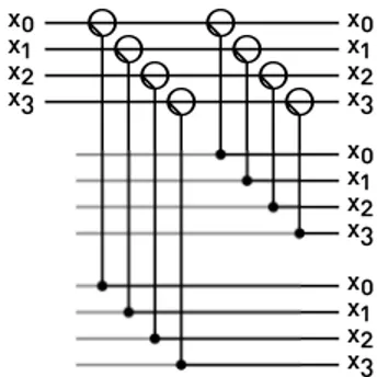
Fanout can be effectively limited to 2 using binary tree switches as described in [1]. For example, ifn = 9, instead of creating8 copies immediately, we construct a binary tree of depth 3, where we create 2, 4, and 8 copies step by step, having a fanout of 2 in every step. Figure 2 shows the binary tree adaptation.
Fig. 2. Binary tree switching. Note that the circles in the switching side depict 1x2 elementary switches.
In the previous examples, the ‘rows’ (horizontal wires) are ordered as below:
(x0,x0,x0), (x1,x1,x1), (x2,· · ·
whereas it is generally more intuitive and efficient to order them as:
(x0,x1,x2,x3), (x0,x1,· · ·
The advantage of implementing the switching stage in this fashion is that there exists a wiring scheme where the total number of columns in the wiring section does not exceed ⌊n
2⌋. A proof is provided in [1]. In this case, binary trees
should overlap, but they can simply be implemented on a grid[1] as shown in Figure 3.
The method to obtain a wiring scheme with ⌊n
2⌋ columns
as described in [1] appeals to cyclic permutation groups. For the example above; the cyclic permutation groups would be as shown below:
Fig. 3. Grid implementation of binary trees. This implementation also groups xiinto blocks.
p = (0123) p2 = (02)(13)
p3 = (0321)
Grouping the numbers obtained by the permutations two by two, one would have the pairs (01), (23), (02), (13), (03), (21). Along with the binary tree implementation depicted in Figure 3, we can implement the wiring step as in Figure 4.
Fig. 4. Wiring step of the one-sided binary tree - crossbar switch.
For even n, obtaining the pairs using cyclic groups is straightforward. However, for odd n, selection of pairs might become tedious. For example, forn = 5, cyclic groups are as shown below:
p = (01234) → (01)(23)(4) p2 = (02413) → (02)(41)(3)
p3 = (03142) → (03)(1)(42)
p4 = (04321) → (04)(3)(21)
Notice that pairs (43) and (13) were not generated, but rather should be constructed by combining the remaining numbers.
In this paper, we present another approach to the problem, which intuitively uses adjacency matrices for representation, and is algorithmically more straightforward. Our method also preserves locality of connections by restricting the intercon-nections between blocks.
II. METHOD
For simplicity and clarity, we will separately handle the two cases for even n and odd n. The reader will easily notice by the end that these two are the reflections of the same approach, only separately defined for mathematical completeness. First, we introduce a notion of equivalence
between pairs of terminals.
Let <i, j > denote the pair between terminals xi and xj.
Two pairs <a, b> and <c, d> are equivalent if and only if (a = c) ∧ (b = d), or (a = d) ∧ (b = c). For example, <0, 3> is equivalent to<0, 3> and <3, 0>. Using this, we can make the following two statements.
Proposition 1. For any a, b and x 6= y, 0 < a, b, < n, 0 < x, y ≤ n
2, the pairs <a, (a + x) mod n> and
<b, (b + y) mod n> cannot be equivalent.
Proof. By the definition of equivalence of pairs, one of the following two cases must be hold.
Case 1:a = b and (a + x) mod n = (b + y) mod n. Then (a + x) mod n = (a + y) mod n, which is possible if and only ifx = y [1], which is a contradiction.
Case 2:a = (b + y) mod n and b = (a + x) mod n. Then a − (b + y) = k1n,
b − (a + x) = k2n
=⇒ −x − y = (k1+ k2)n = −cn
where k1, k2, c are integers. But since 0 < x 6= y ≤ n2,
0 < x + y < n; therefore 0 < c < 1, a contradiction.
Proposition 2. Pairs <a, (a + x) mod n> and <b, (b + x) mod n> cannot be equivalent for any a 6= b and 0 < x < n
2.
Proof. By the definition of equivalence of pairs, sincea 6= b, it immediately follows that these two pairs are equivalent if and only ifa = (b + x) mod n and b = (a + x) mod n. Then
a − (b + x) = k1n,
b − (a + x) = k2n
=⇒ −2x = (k1+ k2)n = −cn
where k1, k2, c are integers. Since 0 < x < n2, 0 < cn < n,
therefore0 < c < 1, again, a contradiction.
In the sequel, we will be using these propositions as we describe our methodology. Also we will make use of adjacency matrices to represent pairs of inputs visually1. In
our diagrams, ‘1’s will be represented by dark cells.
A. Odd n Case
Given that n is odd, all pairs can be defined in the following fashion:
1An adjacency matrix is a binaryn × n matrix in which ‘1’s represent
pairings; a 1 in rowi and column j represents a pairing between inputs i and j.
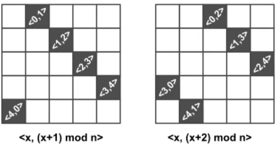
<i, (i + k) mod n>, 0 ≤ i < n, 1 ≤ k < n 2.
For example, forn = 5, the pairs are:
k=1:<0, 1> <1, 2> <2, 3> <3, 4> <4, 0>, k=2:<0, 2> <1, 3> <2, 4> <3, 0> <4, 1>. For a range of 0 ≤ x < n, (x + i) mod n is a diagonal line on the adjacency matrix, as shown on Figure 5.
Fig. 5. Adjacency representation of pairs of inputs.
It follows from Proposition 1 that for different values of k, we always have non-overlapping sets of pairs. In addition, Proposition 2 shows that for a given k, all pairs with the same k are different from each other. Note that, for a given k; the number of <i, (i + k) mod n> for 0 ≤ i < n pairs is exactly n, and each i appears twice in these pairs: once on the left-hand side, once on the right-hand side. For a given k the number of ‘copies’ of xi required is exactly 2; thus,
blocks of x0, x1· · · xn−1 can be grouped two by two. Since
cases for differentk values do not have interconnections, they can be handled separately in parallel.
Another example is shown for n = 7 as in Figure 6. In this case k is between 1 and 3 because n = 7 and 1 ≤ k ≤
1
2(n − 1) = (7 − 1)/2 = 3. Since the adjacency matrix is
symmetric (<i, j>≡<j, i>), all pairs can be depicted in the upper triangle as below.
Fig. 6. n = 7 case. All pairs are shown in the upper triangle.
B. Even n Case
The equation introduced for the odd case is valid for the even case, although it is not sufficient to cover all possible pairs:
<i, (i + k) mod n>, 0 ≤ i < n, 1 ≤ k < n 2.
For n = 6, the exact number of possible pairs is
1
2n(n − 1) = 1
26 · 5 = 15, whereas the definition above
generates n · (n
2 − 1) = 6 · 2 = 12 pairs. The three missing
pairs belong to the case wherek = n 2 = 3.
However, includingk = n
2 to the boundary of the equation
above would violate the conditions defined fork in Proposition 2. To demonstrate, letn = 6 and k = 3. The pairs generated are as follows:
<0, 3> <1, 4> <2, 5> <3, 0> <4, 1> <5, 2> In this case, all pairs appear twice; once in order, then in reverse, such that <a +n
2, ((a + n 2) + n 2) mod n > = <a +n 2, a> ≡ <a, a + n 2>, when k = n 2. The problem is solved if0 ≤ a < n
2 instead of0 ≤ a < n, in which case the
modulo operator disappears, and the pair definition becomes simplified as <i, i +n
2>.
Then the two subsets that cover the even n case are as follows: <i, (i + k) mod n>, 0 ≤ i < n, 1 ≤ k < n 2, <i, i +n 2>, 0 ≤ i < n 2. Since k are different, Proposition 1 shows that these two subsets never overlap. Set 1 has n(n
2 − 1)
elements, and set 2 has n2 elements; adding up to (n + 1)(n 2) − n = 1 2n(n + 1) − 1 22n = 1 2n(n − 1)
unique elements; covering every necessary pair.
Figure 7 shows how pairs are generated for n = 8. The rightmost figure shows the second set (k = 8
2 = 4 case).
Fig. 7. Pair generation for evenn. The rightmost figure depicts the k = n/2 set.
Note that the special definition provided for the k = n 2
case, prevents the last 4 cells to be spanned twice.
C. Wiring
The actual wiring of the generated pairs is described in the following section.
For even n, wiring of the second set is trivial, because the first half of inputs connect to the second half. Since there are
n
2 wires, the number of columns is exactly ⌊ n 2⌋ =
n 2. Only
one block is necessary and sufficient for the wiring of this set. An example is shown in Figure 8 for n = 8.
Fig. 8. Wiring of the block handling thek = n/2 case for n = 8.
Having handled the special case for even n, the remaining pairs are identically defined for odd and even n:
<i, (i + k) mod n>, 0 ≤ i < n, 1 ≤ k < n 2.
In order to get rid of the modulo operator and represent all pairs < a, b > in the upper triangle such that a < b, the definition above should be separated into two subsets as shown below for each k (1 ≤ k < n
2):
< i, (i + k) > for0 ≤ i < n − k, < (i + k − n), i > for n − k ≤ i < n. The second subset can also be written as follows:
< i, i + n − k > for 0 ≤ i < k. k < n
2 =⇒ k < n − k; therefore the range for i in the
second set is a strict subset of the range for i in the first set. Since the first set uses the first copies of the terminals, the second set should strictly be placed on to the second block (recall that exactly two blocks are allocated for each value of k). That is, the first k values for i in the first set are forced to belong to the first block. Since these pairs are defined as <i, (i + k)>; the xk· · · x2k−1 terminals in the first block are
used as the destination ports; therefore these connections are made in the second block, and so forth.
The resulting distribution of connections can be formalized in the following manner:
• The second set always belongs to the second block. • For a pair in the first set<i, (i + k)>, if ⌊ki⌋ mod 2 = 0,
put the pair in the first block, otherwise put it in the second block.
Recall that these formulations are defined for a fixed k, and should be repeated for every k in range. Figure 9 is the resulting circuit for n = 8. The condition for k = 3 is handled separately and uses only one block. The other blocks are clustered in two, and have no interconnections.
Fig. 9. Complete wiring scheme for n=8. Each cluster of inputs correspond to a separate value of k, and these clusters have no connection in between.
For demonstration purposes, pairs generated by the second set are shown on the right-hand side.
A verbal guideline for the approach can be provided as follows:
• Given a k, insert the first k pairs
(<0, k>,<1, k + 1>,· · · ,<k − 1, 2k>) into the first block.
• Insert the nextk blocks to the second; then the following
k into the first...
• Continue this process until the first set is exhausted. • Insert every item in the second set into the second block. • Repeat steps above for everyk.
• If n is an even number, consider the k = n/2 case
separately as described above.
As long as the first-second block selection process is respected, regardless of the order in which the pairs are inserted, no collisions can occur. Finally, it is not difficult to prove that the number of columns does not exceed ⌊n
2⌋ in
this scheme.
III. CONCLUSION
We presented an algorithm to connect all pairs ofn termi-nals in an n-terminal one-sided, binary-tree switch in ⌊n/2⌋ columns of wiring. We have implemented and tested this algorithm in Java. The implementation provides an .svg vector output as well as an ASCII console representation of the wiring scheme. The code for the algorithm is available at https://github.com/kubuzetto/crossbarWiring/.
[1] A. Yavuz Oruc¸. One-sided binary-tree-based crossbar switch fabrics. Invention Disclosure. University of Maryland, College Park. PS-2014-57. Apr. 9, 2014.