Proper orthogonal decomposition for reduced order modeling: 2D heat flow

Proper Orthogonal Decomposition for Reduced

Order Modeling: 2D Heat Flow-

Mehmet Onder Efe Hitay Ozbay

Collaborative Center o f Control Science Department of Electrical Engineering

The Ohio State University Columbus, OH 43210, U.S.A.

E-mail: onderefe@ieee.org

Dept. of Electrical & Electronics Eng. Bilkent Univ., Ankara TR-06533, Turkey

on leave from Dept. of Electrical Eng. The Ohio State University E-mail: ozbay@ee.eng.ohio-state.edu

Abstract-Modeling issues of infinite dimensional systems is studied in this paper. Although the modeling problem has been solved to some extent, use of decomposition techniques still pose several difficulties. A prime one of this is the amount of data to be processed. Method o f snapshots integrated with POD is a remedy. The second difficulty is the fact that the decomposition followed

by a projection yields an autonomous set of finite dimensional

ODEs that is not useful for developing a concise understanding of the input operator of the system. A numerical approach to handle this issue is presented in this paper. As the example, we study 2D

heat flow problem. The results obtained confirm the theoretical claims of the paper and emphasize that the technique presented here is not only applicable to infinite dimensional linear systems hut also to nonlinear ones.

1. INTRODUCTION

Although the applications o f Proper Orthogonal Decomposi- tion (POD) particularly focus on the extraction o f coherent and dominant modes available in aerodynamic flows, the problem of tackling with huge amounts of data and technical difficulties in the obtained modcl constitute bamers between the stipulated efforts and the thorough understanding of the process, [1-6].

For this reason, we study the modeling problem that addresses the above mentioned difficulties appropriately on a 2D, simple, and a linear dynamics, namely the heat flow. The goal o f

the paper is to introduce how the data is obtained, how the external stimuli enter into the dynamics, and how the data set is processed so as to obtain

a

set of orthogonal basis, and finally, how the external stimuli is made explicit in an autonomous set

o f ODES.

Modeling of systems displaying spatial continuum requires a careful consideration since the physical process under in- vestigation is an infinite dimensional one due to the spatial continuity. Efforts in understanding the behavior of such systems have particularly focused on the low dimensional models capturing the essential behavioral properties with a few Ordinary Differential Equations (ODEs). This has been done by using modal decompositions such as Proper Orthogonal Decomposition (POD) and Singular Value Decomposition (SVD). Although neither the decomposition techniques nor the infinite dimensionality are new issues in this field, obtaining a model having the boundary conditions as extemal inputs

is a major problem in the POD and SVD methods. More

explicitly, these approaches result in models where extemal control input appears in the dynamical equations implicitly, and this is not very useful for controller design. Another difficulty is the presence o f modeling uncertainties, which stem from varying internal parameters or hypotheses that are not thoroughly valid. For the heat transport process, imprecise knowledge on thermal ditksivity parameter is a good example to study uncertainties.

The use of decomposition techniques in modeling of spa- tially continuous systems has extensively been studied in the field o f aerodynamic flow control problems, [1-4]. Since the dynamics of the process under investigation is governed by Navier-Stokes equations, obtaining closed form solutions are very difficult and the modeling studies particularly focus on the real timc observations from the process. For systems having two or more spatial dimensions, the POD technique has been utilized with the aid of snapshots method, [I-21. Altematively, for single dimensional processes, the same modeling procedure can be followed by exploiting the SVD technique.

Procedurally, in both o f them, if the numerical data contains coherent modes, the expansion accurately describes the tem- poral modes and the spatial components distributing them over the physical domain o f the process. Furthermore, the orthogo- nality o f the basis functions, which describe the spatial proper- ties, helps in finding a set o f ODEs synthesizing the temporal modes. Although the algorithmic part seems straightforward, the final form of the ODES depicts an autonomous system having no extemal input. At this point, several modifications are needed to separate the effect of boundary conditions, which constitute the inputs exciting the process. 2D heat transport problem is therefore a good candidate to study how modeling issues are addressed.

A number of variations of this problem has been taken into consideration in former studies, [5-71. Atwell et al [S-61, have considered 2D heat transport problem with control input explicitly available in the Partial Differential Equation (PDE). The thermal diffusivity parameter has been taken as a known constant and several control strategies have been assessed with the modeling results o f POD approach. In [6], the design has been discussed from the computational point o f view.

ports the design of time-optimal boundary control, [7]. It is emphasized in [7] that the tinie-optimal control has the bang- bang property, and the solution has been postulated by the techniques of Hilbert spaces. Rosch [8], views the character- ization of boundary condition as an identification problem, and presents an iterative approach to meet the conditions of optimality.

Although the techniques of functional analysis suggest several solutions to the problem at hand [9], the presented technique here can be generalized to a variety of systems dis- playing arbitrarily complicated behavior. This fact is intimately related to the observation-based nature of the approach.

The way this paper differs from what have been appeared in the literature is to demonstrate how a low-order model having an external control input is derived. In the sequel, the details will be presented in the following organization: The second section presents the POD technique and its relevance to the modeling strategy. In the third section, development of the reduced order model for the 2D beat flow is analyzed. The fourth section presents the results and the concluding remarks are given at the end of the paper.

11. PROPER ORTHOGONAL DECOMPOSITION

Consider the ensemblc

Ui(z,

y) i = 1 , 2 , . . .

,

N . Appar- ently, every element of this set corresponds to a snapshot observed from a process, say for example, the 2D heat equation u t ( z ; y, 1 ) : c2 (uZz(z, y, t ) t uY,,(z; y? t ) ) , where

c is constant.

The goal is to find an orthogonal basis set letting us to write the solution as

A'

u(z:y,t)

=

X%(t)d&>U)>

(1)

z = 1

where a t ( t ) is the temporal part, and &(z, U) i s the spatial part. It will later be clear that if the basis set {$i(z,y)}t*J=l is an orthogonal set, then the modeling task can exploit Galerkin projection technique.

Step 1. Start calculating the N x iV correlation matrix L, the ( i j ) ' h entry of which is Lij := (Ui,Uj)n, where (., .)n is the inner product operator defined over the spatial domain (0) of the process.

Step 2. Find the eigenvectors (denoted by

vi)

and the associ- ated eigenvalues ( X i ) . Sort them in a descending order in terms of the magnitudes of X i . Note that every ut is an

N

x 1 vector satisfying

$vi

=

k,

here, for simplicity of the exposition we assume that the eigenvalues are distinct.

Step 3. Construct the basis set by using Let us summarize the POD procedure.

N

d i h Y )

= CUtjU,(Z,Y), ( 2 )

j-1

where w i j is the j t h entry of the eigenvector wi, and i = 1 , 2 , ..., rank(L). It can be shown that ($,(z,y),$j(z,y))n = 6, with 6, being the Kronecker delta function.

Remark 1. Notice that the basis functions are admixtures of the snapshots.

Step 4. Calculate the temporal coefficients. Taking the inner product of both sides of ( I ) with $i(z,y), the orthogonality lets us have

adto)

= ($J.r,Y),u(z,Y,to))n

= ( $ i ( Z , Y ) : Ut,)n, (3)

Without loss of generality, an element of the ensemble { U i ( % > y ) } z l may be U(z,y,to). Therefore, to generate the temporal gain

( s ( t ) )

o f t b e spatial basis &(z,y), one would take the inner product with the elements of the ensemble with sampled forms of the basis functions.

Remark 2. Notice that the following hold true:

N M

i=l i=l

= Xk

Apparently, the temporal coefficients satisfy orthogonality properties over t E {tl, tz, . . .

,

t N }

In the next section, we demonstrate how the boundary condition is transformed to an explicit control input in the ODES.

111. R E D U C E D O R D E R MODELING

Consider the heat conduction problem over the spatial domain Cl := (z,y) E ( O , l ] x [O,l]. Truncate the sum in

( I ) after some certain integer, say M , and assume that the modes from

M

+

1 to w are reasonably small in magnitude such that we can write the following:

M

U ( Z , Y , t ) = C n i ( t ) $ i ( s > Y ) . (4)

i = l

The solution above must satisfy the PDE, i.e. we get

2=1 ,=1

where <,(z,y) = $ $ ( ~ , y ) , ~ t $2(z,y)yy. Clearly taking the inner product of both sides with & ( r , y) yields

M

where k = 1: 2 , .

.

.

,

M .

Apparently no matter what the boundary conditions, the above representation contains the

effect of them implicitly. To overcome this problem, denote the set of points, at which boundary excitations are independently suecified, bv .~ 8R. The underlvinr idea in develouine the . I . -

-

dynamic model is the following fact:

(&(z,Y);Ci(z,y))n = ( h ( z , ~ ) , C t ( ~ ; ~ ) ) a n

+

( 4 k (z, Y

1,

c

(2, Y) h \ a n I (7)

which basically corresponds to the repartitioning of the domain by changing limits of a Riemann integral computed over a non- intersecting subdomains embodying the domain of the original integral when they are united.

Define

an

:= { ( 0 , 0 ) ~ ( 0 , 1 ) , ( 1 ~ 0 ) ~ ( 1 , 1 ) } . Thismeans that the external stimuli enter from the comers of the domain. In other words, the dynamic input will have four inputs denoted by yoo,yo1,ylo and 711. Clearly, in this notation the first index

stands for z and the second stands for y.

Denote the solution observed when */oo(t)=goo(t) with other inputs are equal to zero as uoo(z7 y: t ) with goo(t) being an arbitrarily chosen test signal. Perform the POD procedure to obtain a solution in the form of (4). Repeating the same procedure till every element of the set a R is contained, one would end up with the following solution when each input assumes arbitrarily chosen values,

p=o q=o i=l

which is the result of the superposition principle. Note that for nonlinear PDEs, this expansion would not bc valid.

Now assume that the system is excited only from ( x ; y) = (0,O) entry. Since the solution in (4) must be satisfied also on 8R, this lets us write the following,

i = l

where p and q assume values either zero or one. Notice that the manipulations in (9)-(11) are for the single excitation from (z, y) = (0,O). Therefore if p = 0, q = 0, the expressions

(10) and (I 1) become identical. However, other combinations o f p and q stipulate that ypq(t) may have a nonzero spatial gain (See (It)) although the ypq(t) is identically equal to zero.

Considering (7) in (6) and using the above equation for every p and q would result in the dynamical system corre- sponding to the described excitation configuration.

where

p=o q=o

The model above can he written in the well known state space form,

-

koo(t) = AoOqoo(t)

+

B o o y ( t ) -

(13) where

y

=

(

700 701 710 YII

)

, and

Biy

= c2Cio(p, U)

with i = 2 p t q t 1. The row vector

C(z,

y) is apparently the vector of 2D basis functions calculated at given points z and y and for given excitation conditions, i.e. 00 for this case.

Clearly, the above model bas M states and four inputs. In order to obtain the full representation, the procedure described in (9)-(13) must be repeated for every y p q ( t ) to obtain the individual components of (8).

Remark 3. Considering (12) and (13), it is apparent how the dynamical model is affected from the uncertainties on the thermal diffusivity parameter e.

Let U ( z , y l s ) :=

C

{u(z,y,s)}, UPq(z,y;s) :=

L

{ P ( z , y , s ) } and r p q ( s ) := L {ypp(S)} with

C

being the Laplace transform operator. In the view of the analysis presented, the total system can be expressed as follows

no

(z:Y,t) = COO(z>Y)cPo(t), T

1 1

where In a similar fashion, one should investigate the spa-

{ ( O , l ) , ( l , O ) , (l,l)}. Performing this would simply let us

tial gain associated with other inputs, i.e. (z,y) E 1 1

generalize (10) as follows:

Umn(z,y>s) = ~ l G ~ ( z , y , s ) T p q ( s ) . (15) p=o q=o

IV. M O D E L I N G RESULTS

According to the described procedure, several tests have been done. The PDE has been solved by using Crank- Nicholson method (See [IO] for details), with a step size of 5 msec. The initial thermal distribution is taken as zero everywhere and the thermal diffusivity constant is set as c = 0.4. In order to form the solution, a linear grid having N , = Nu = 25 points in 2-direction and y-direction respectively. According to the above parameter values, a total of 201 snapshots embody the entire numerical solution, among which a linearly sampled Ai = 21 snapshots have been used for the POD scheme. Although one may use the entire set of snapshots, it has been shown that a reasonably descriptive subset of them can he used. In the literature, this approach is called method of snapshots, which significantly reduce the computational intensity of the overall scheme, [I-21. Once the modes have been obtained, we truncated the solution at

hf = 5 , which represents (in average)

According to the above settings, the inner product seen in (6) is calculated as follows:

f

in which we calculate the derivatives numerically.

The system has been stimulated from every comer, with one-at-a-time basis. For collecting data, we used several test signals given as

g p 9 ( t ) = 0.1 t Pexp(-Gt) sin(8at) gp9(t) = sin(2at)

g,,(t) = 1 -exp(-6t)

g*&) =

4'

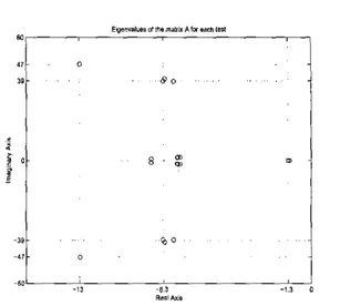
(1 7)

where subscript p q indicates the chosen comer. For each case. the basis surfaces change very slightly and this influences the content of the matrices in (13). Checking the eigenvalues of the matrix A is an indicator of the similarity between each case. This is illustrated in Figure 1, in which the eigenvalues form individual clusters.

In order to construct the dynamic model, the matrices obtained for different test conditions at a chosen comer have been averaged. To compare the overall solution with the numerically obtained data, we choose the following boundary excitations, which are applied simultaneously:

yoo(t) = sin(2at) y o l ( t ) = -sin(3at) y l o ( t ) = sgn(sin(2at))

y l l ( t ) = 1 - exp(-6t). (18)

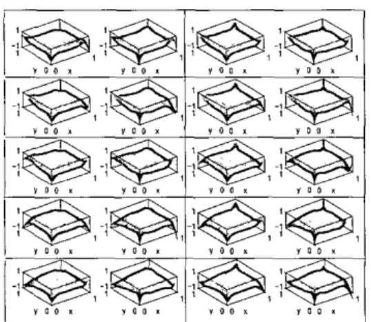
The results for this case are depicted in Figure 2. Every pair in this figure represent the numerical solution (on the left) and

~

Fig. I, Clusters of eigenvalues appear as the procedure is repeated for different test conditions. A test signal is chosen and an input point is chosen to complete one experiment. The figure depicts 16 experiments and 80 data points.

the reconstructed solution (on the right). The pairs in the first line stand f o r t = 0.lsec. (on the lee) and t = O.2sec. (on the right) and the rest includes solutions sampled at the same rate till t = lsec.

Fig. 2. A comparison of the solutions generated by the numerical solver and the low-order dynamic model. The frequency ranges of the test conditions and the validation are similar.

It is clear from Figure 2 that the surfaces at every cell are reasonably similar to each other. This result confirms the analytical claims and validates the method described to separate the effect of control terms.

Remark 4. It should be noted that the modes of the infinite dimensional system have been excited by a set of test signals (17), and the result has been validated on

a

similar set of boundary conditions (19). The answer to the immediate question "why" is as follows: The model is valid dominantly for the frequency range covered by the test signals. If one wants to cover a wide range of frequency spectrum, then this would first require smaller step size for the PDE solver and much longer time to obtain a representative set of snapshots.

On the other hand, the POD procedure will filter out some of the high frequency content. The reader should notice that the underlying idea of the POD procedure is to reconstruct the solution from its samples (snapshots), however, a good reconstruction can be performed only when the solution is dominated by coherent modes, which implies relatively low frequency content of the entire solution. A good comparison is presented in Figure 4 for the following boundary conditions:

roo(t) = sin(20rt)

Tol(t) = sin(2rt) Tio(t) = sgn(sin(l4st))

n l ( t ) = -sin(30rt)> (19)

in which the frequency range is increased approximately about ten times for all comers except

rol(t),

which is kept in the frequency range of the modeling stage so that the difference will be clear. Refemng to Figure 3, it is apparent that the evolution of the comer signals are so fast that the reduced order model cannot reconstruct the solution around them, however around the comer

n o ( t ) ,

the reconstruction is unsurprisingly good. This result simply validates our remarks.

Fig. 3. A comparison o f the solutions generated by the numerical solver and the low-order dynamic model. The frequency ranges o f the test conditions and the validation are not similar.

Remark 5. The dissimilarity observed in the second case raises the following question: Does the percent energy de- scribed earlier depend upon the frequency content of the test signals? The answer is apparently yes. Basically, a model is valid in the frequency range of data that leads to the model. The degree of confidence decreases as the overlapping between the model derivation conditions and the operating conditions becomes dissimilar. Altematively, one can interpret this as follows: Fixing the number of modes

(At)

(or equivalently fixing the energy level) cannot lead to the reconstruction of the information hidden in the modes

A4

+

1 to N .

V. CONCLUSIONS

I

Many physical phenomena, such as areodynamic flows, flex- ible object dynamics, and heat transport have infinitely many

dynamical modes describing the entire behavior when they are considered collectively. In this paper, the reduced order mod- eling of 2D heat equation is considered. The physical domain is a square plate, and the excitation enters into the system from the comers of the plate. The algorithmic approach has been shown to be capable of capturing the dynamically significant modes of the solution. Once the number of modes is decided, the procedure yields a set of autonomous ODEs. We present a method to separate the external stimuli from these ODEs. The described approach has been shown to be successful in terms of the similarity between the numerical solution and the solution based on the low-dimensional model. We observed that the widely accepted form of the realization performance, which is the percent energy captured is a frequency-variable quantity, and it does not constitute a globally valid measure of realization performance. As long as the data is a representative for the operating conditions, the results are highly promising in the sense of extending the modeling and separation techniques for more difficult and nonlinear cases, such as for aerodynamic flows, which constitute the ultimate goal of this research.

ACKNOWLEDGMENTS

This material is based on research sponsored by Air Force Research Laboratory, Agreement no: F33615-01-2-3154.

The authors would like to thank Prof. M. Samimy, Dr. J.H. Myatt, Dr. J. DeBonis, Dr. M. Debiasi, X. Yuan and E. Caraballo for fruitful discussions in devising the presented work.

R E F E R E N C E S

[ I ] S.S. Ravindran, A reduced order approach for optimal control o f fluids using proper orthogonal decomposition. Int. J. for Numerical Methods

in Fluids, 34, 425-488 (2000).

121 H.V. Ly and H.T. Tran, Modeling and control of physical pmcesses using proper orthogonal decomposition. Mathemoricol and Computer

Modelling ~$Dynamicol Systems, 33, 223-236 (2001).

[3] S.N. Singh, J.H. Myatt, G.A. Addington, S. Banda and J.K. Hall,

Optimal feedback control of vortex shedding using proper orthogonal decomposition models. Trans. of rhe ASME: J o/ Fluids Eng., 123. 612-618 (2001).

[4] P.N. Blossey and J.L. Lumley, Reduced-order modeling and control of near-wall turbulent flow. Proc. of the 38th Conf. on Decision and Control, 2851-2856, Phoenix, Arizona, U.S.A. (1999).

[5] J.A. Atwell and R.R. King, Proper orthogonal decomposition for reduced basis feedback controllers for parabolic equations. Mnfhemafical nnd

Computer Modelling. oJLIymmica1 Systems, 33, 1-19 (2001). [6] I.A. Atwell and R.B. King, Computational aspects of reduced basis

feedback controllers for spatially distributed systems. Proc. of the 38th Conf. on Decision and Control, pp. 4301-4306, Phoenix, Arizona, U.S.A. [7] V.J. Mizel and T.I. Seidman, An abstract bang-bang principle and time- optimal boundary control of the heat equation. SIAM Journal on Control and Optimizaiion, 35 (4), 1204-1216 (1997).

[SI A. Rosch. Identification o f nonlinear heat transfer laws by optimal control. Nirmerical Functional Analysis and Optimizoiion, 15 ( 3 4 417- 434 (1994).

[9] R.F. Cumin and H.J. Zwan, An Introduction to Infinite-Dimensional Linear Systems Theory, Springer-Verlag, New York, 184-189 (I 995). [IO] S.J. Farlow, Partial Differential Eqiations far Scientists and Engineers,

Dover Publications Inc., Ncw York, 317-322 (1993). (1999).