Online anomaly detection under Markov statistics with controllable type-I error

Online Anomaly Detection Under Markov Statistics

With Controllable Type-I Error

Huseyin Ozkan, Fatih Ozkan, and Suleyman S. Kozat, Senior Member, IEEE

Abstract—We study anomaly detection for fast streaming

temporal data with real time Type-I error, i.e., false alarm rate, controllability; and propose a computationally highly efficient online algorithm, which closely achieves a specified false alarm rate while maximizing the detection power. Regardless of whether the source is stationary or nonstationary, the proposed algorithm sequentially receives a time series and learns the nominal at-tributes—in the online setting—under possibly varying Markov statistics. Then, an anomaly is declared at a time instance, if the observations are statistically sufficiently deviant. Moreover, the proposed algorithm is remarkably versatile since it does not require parameter tuning to match the desired rates even in the case of strong nonstationarity. The presented study is the first to provide the online implementation of Neyman-Pearson (NP) characterization for the problem such that the NP optimality, i.e., maximum detection power at a specified false alarm rate, is nearly achieved in a truly online manner. In this regard, the proposed algorithm is highly novel and appropriate especially for the applications requiring sequential data processing at large scales/high rates due to its parameter-tuning free computational efficient design with the practical NP constraints under stationary or non-stationary source statistics.

Index Terms—Anomaly detection, efficient, false alarm, Markov,

Neyman-Pearson, NP, online, time series, type-I error.

I. INTRODUCTION

D

ETECTION of anomalous patterns is of great interest in signal processing [1]–[4] and machine learning [5] since the irregular data due to an anomaly often detrimentally affects the target application and might even require special actions in certain scenarios [5]–[7]. For instance, a hacked computer/mo-bile device produces suspicious network traffic [8]; or an il-legal U-turn in an intersection scene creates anomalous video Manuscript received March 30, 2015; revised August 28, 2015 and November 10, 2015; accepted November 14, 2015. Date of publication November 30, 2015; date of current version February 09, 2016. The associate editor coordi-nating the review of this manuscript and approving it for publication was Dr. Ruixin Niu. This work was supported in part by The Scientific and Technolog-ical Research Council of Turkey (TUBITAK) under Contract 113E517 and in part by the Turkish Academy of Sciences Outstanding Researcher Program.

H. Ozkan is with the Department of Electrical and Electronics Engineering, Bilkent University, Ankara 06800, Turkey. He is also with the UGES Di-vision at Aselsan Inc., Ankara, Turkey (e-mail: huseyin@ee.bilkent.edu.tr; huozkan@aselsan.com.tr).

F. Ozkan is with the Department of Information Systems, Middle East Tech-nical University, Ankara 06800, Turkey (e-mail: fatih.ozkan@metu.edu.tr).

S. S. Kozat are with the Department of Electrical and Electronics Engi-neering, Bilkent University, Ankara 06800, Turkey (e-mail: kozat@ee.bilkent. edu.tr).

Color versions of one or more of the figures in this paper are available online at http://ieeexplore.ieee.org.

Digital Object Identifier 10.1109/TSP.2015.2504345

data [3]; or an anomalous pattern in the electricity consump-tion data of a factory should definitely raise concerns [9]. Sim-ilarly, visual occlusions generate unpredictably irregular video data and reduce the object recognition rates [10]. In this paper, we study the anomaly detection problem for the temporal data in the online setting and propose a novel and computationally highly efficient online algorithm. The proposed algorithm se-quentially receives a time series, learns -in an online manner-the nominal attributes in manner-the data and detects manner-the anomalous sub-sequences. We use the Neyman-Pearson (NP) characterization [11] for the anomalies and nearly achieve a constant control-lable false alarm rate with maximum possible detection power regardless of whether the source is stationary or non-stationary. The proposed algorithm is able to process data in real time at ex-tremely large scales/high rates with linear complexity in the size of the stream. Moreover, we do not require parameter tuning to match the desired rates even if the source statistics change.

There exists an extensive literature on anomaly detection [1], [3], [5]–[7] and the problem is studied under different nomencla-ture depending on the anomaly types such as novelty detection [2], [12], [13], outlier detection [4], [14], [15], one class learning [16], [17], intrusion detection or fault detection [18]. However, as the first time in the literature, we focus on online anomaly detec-tion in stadetec-tionary or non-stadetec-tionary fast streaming temporal data with online controllability of the Type-I error that maximizes the detection power without requiring parameter tuning. Thus, the presented study considerably differs from the literature. We con-sider that the controllability of the false alarm rate is a crucial capability especially in the context of anomaly detection since anomalies in general draw attention and provide actionable in-formation. In this regard, a number of false alarms more than a bearable rate is clearly frustrating and hence potentially risks the practicality of the algorithm [19], [20]. For this reason, we study the problem in the binary hypothesis framework by using the NP formulation [11], where we explicitly bound the false alarm rate (i.e. minimizing Type-I error) while achieving the maximum de-tection power (i.e. minimizing Type-II error). Although the NP approach is successfully applied to anomaly detection [4], [19], [20], the online implementation of the NP solution has been left unexplored. Furthermore, the existing batch NP solutions are typically based on the assumption of independent and identi-cally distributed (i.i.d.) observations, which hardly holds in the case of temporal observations, where the data is typically highly correlated in time and non-stationary. In contrast, we model such intrinsic correlations via Markov models without assuming stationary source statistics.

Our method falls in the category of statistical anomaly detec-tion with modeled nominal densities [5], [21], where an anomaly 1053-587X © 2015 IEEE. Personal use is permitted, but republication/redistribution requires IEEE permission.

is an observation that is (suspected to be) not generated by the assumed nominal stochastic model. Accordingly, we learn a parametric model (a birth-death type discrete time Markov chain in this study) for the time series data; and our anomaly detection approach is to optimally test (in the sense of NP constraints) whether the sufficient statistics of a new sequence is consis-tent with the learned model. A popular approach in statistical anomaly detection is to consider the distance from a suspicious instance to the nominal set of data. In [22], if the ’th minimum distance is sufficiently large, then an anomaly is declared. The rankings of these ’th distances are used in [23] to bound the number of false alarms in a computationally relatively more efficient manner. Such rankings have shown in [20] to be an asymptotically consistent estimator for inclusion in the Min-imum Volume (MV) set, which is the complement of the optimal decision region for anomalies in the NP formulation when the anomalies are assumed to be uniformly distributed, cf. [19]. The method in [20] impressively avoids the explicit calculation of the MV set but rather calculates the sufficient membership in-dicator via the ’th rankings. Another method is the Geometric Entropy Minimization (GEM) [24], which compares a test instance with only the most concentrated subset of the nominal training data that is asymptotically convergent to the MV set.

We also use the Minimum Volume (MV) set approach to de-tect anomalies in temporal data. However, our goal is to obtain a computationally scalable algorithm while maintaining the NP optimality, i.e., Type-I error controllability with maximum detection power. These methods [19], [20], [22]–[24] are batch processing methods, i.e., not online, without any update strate-gies; and they are computationally too demanding for real time processing in fast streaming data applications. For instance, the methods [20], [22], [23] require pair-wise distance calculations and sorting to obtain the rankings and essentially to order the likelihoods, which typically results in quadratic complexity in the data size (and which are even further complex, if one also considers the model updating for the new data arriving at each time). The method in [19] is appropriate only for the batch processing and only when the batch data is of relatively small number of instances and of low dimensionality, e.g., 2-dimen-sional, due to the -for instance- computationally heavy and not scalable dyadic-tree implementation. Similarly, the GEM method [24] is computationally not tractable, i.e., impractical; and its tractable version (presented as another algorithm in [24]) still requires computationally heavy batch processing without the original statistical guarantees. Thus, one can hardly use such methods in our framework of sequential data processing at large scales/high rates, although they are impressive batch processing techniques. On the contrary, instead of such distance calculations and orderings, we directly approximate the distri-bution of the likelihoods under the general Markov models for temporal data and analytically calculate the desired quantile for the MV set. This allows a computationally highly efficient and online implementation of the NP approach with controllable Type-I error and maximum detection rate. Moreover, we do not require (like [20] and unlike others) parameter tuning to match the desired false alarm rate and also, we do not assume (unlike these methods) stationary data source.

The goal in this paper is to detect anomalous subsequences in a time series. This instance of the problem for temporal data

(not in the i.i.d. batch setting like [5], [19], [20]) has also been considered, cf. [25]–[36] and the references therein. However, most studies do not address the problem in the online setting and they assume stationary source statistics [6], [7]. An anomaly score is assigned to each fixed length subsequence using the pair-wise distances among all possible such subsequences in [25] and the detection is based on the magnitude of the anomaly score. Several approaches [27]–[30] are then proposed to relieve the computational burden of the pair-wise distance calculations such as tree representations and prunings [26], local hashing [27] and Haar transform [29], [34]. Instead of the standard Eu-clidean distance, a compression based similarity measure is also investigated in [31], [32]. Several other methods exists, which consider unevenly sampled stochastic processes [33] as well as differently defined anomalies [7], [35], [36]. Despite the impres-sively efficient implementations (for instance [26], [30], [32], [36]), the model free setting along this line of research requires to investigate pair-wise relations or extract/apply complex fea-tures/transformations. Hence, their solutions are essentially not appropriate to process large scale data in real time due to their computationally heavy requirements. In contrast, we exploit the availability of the data in huge amounts and therefore the ability to precisely estimate a general Markov model, which conve-niently avoids such complex computations. Additionally, unlike these discussed studies, we ensure the false alarm controllability without parameter tuning even in the case of the non-stationary sources.

Markov models are also frequently used for anomaly detection in temporal data [3], [5]–[7], [37]–[41]. The unknown Markov model parameters are first estimated in the training phase and thereafter, if the probability of a test instance is sufficiently small compared to a threshold, then an anomaly is declared in these studies. In [38], this approach is successfully demonstrated for first order Markov models, where the extension to the desired generality with higher order is straightforward. Efficient repre-sentations for large alphabet sizes is considered in via a suffix tree used in conjunction with a finite state automata in [41]; and also an extended finite state automata in [39], [40]. In [37], anomalies are defined as labeling errors in case of the hidden Markov models and their effects on state recognitions are inves-tigated. In the video anomaly identification [3], the pixel based motion patterns are modelled under first order Markov statistics and the sufficiently unlikely patterns are labeled anomalous. Markov models are generally efficient and can be extended to online implementations. However, it is difficult to related the threshold parameters in these studies to the false alarm rates, and even once tuned correctly; re-adjustments is necessary, if the source statistics change. In contrast, our online algorithm does not require parameter tuning, i.e., it is parameter-tuning free, regardless of the stationary or non-stationary source statistics. We also guarantee to match the specified bearable false alarm rate (constant false alarm rate) while operating on the fast streaming input data in a truly online manner at the maximum possible anomaly detection power.

We provide the problem formulation in Section II. After the proposed method is described in Section III, we present our on-line algorithm in Section IV. We demonstrate the performance of our algorithm in Section V. The paper concludes with final remarks in Section VI.

II. PROBLEMFORMULATION

We first concentrate on the stationary sources, then proceed to non-stationary settings in Section IV and present examples in Section V.

We consider a real valued, bounded, stationary and ergodic discrete time stochastic process1 _{, i.e., with the}

range space being (arbitrarily large and) finite, and . Our goal is to detect anomalous subsequences, i.e., windows, in a given realization from the process . For this purpose, we define a (sliding) window sequence

of window length at a time with .

Note that the definition of the window sequence depends on the time , which is not shown in “ ” for notational simplicity. Then, we decide whether the sequence is statistically con-sistent with the underlying process , i.e., anomalous, or not. An anomaly often occurs due to an external factor over-writing the actual data or an abrupt change in the source statistics [5], [10]. Since the characteristics of such an external factor or a sudden change cannot be predicted beforehand, it is reasonable to assume that an anomaly can be at any point in the observation domain, i.e., it is uniformly distributed [10], [19], [20]. To detect anomalies of this kind, we formulate the problem in the Neyman-Pearson (NP) testing framework, where one minimizes the miss rate at the cost of a pre-specified false alarm rate . The NP test in this regard declares an anomaly when

(1) such that

(2) where is the probability mass function (p.m.f.) for a nom-inal window from and is the length of the se-quence . We point out that:2_{if -for instance- the real-valued}

mother sequence is allowed to span the real line, i.e., , then the summation in (2) must be replaced with an integra-tion, which would not affect our derivations or our development. However, since we will use quantization in the amplitudes in our signal model later, it is convenient here to use a finite range space and hence a summation in (2) without loss of gen-erality. Since is random, the log-likelihood

1_{Bold font types are used to indicate multiple quantities such as a sequence,}

vector or matrix. Upper case letters are used to indicate a matrix or random quantity. For instance, is a sample, is the sequence, is the stochastic process; is a scalar, is a random variable, is a vector and is a matrix. Further distinction is clear from the context with no confusion. is the in-dicator function such that , if is TRUE; and 0, otherwise. is the size of a set or determinant of a matrix or an absolute value depending on the argument. All listings of the form generates a column vector and gen-erates a set. is the transpose of a matrix . is the floor operation for a scalar , i.e., . We use the “ ” notation to refer to corresponding cases respectively, i.e., and . All logarithms are natural logarithms.

2_{Note that the summation in (2) is over all possible windows of length ,}

i.e., ; therefore, the threshold depends on . Since the process is stationary, the p.m.f. accepts a common form across all windows of

but its form depends on the window length. Although “ ” would be a proper notation, we drop the subscript for simplification in notation.

is also random with the corresponding density3 _{. Then, the}

same test in (1) can also be written in the log-likelihood domain as

(3) such that

This test (the Neyman-Pearson (NP) test) is the “most pow-erful” in the sense that it yields the highest detection rate at the false alarm level when the anomalies are uniformly distributed [10], [19], [20]. Our aim is to devise computationally efficient online (with linear complexity in the number of instance) NP tests for anomaly detection for time series.

III. ANOMALYDETECTIONUNDERMARKOVSTATISTICS The problem described in Section II requires one to determine not only the log-likelihood but also the density of the log-likelihood in addition to the threshold . For this purpose, we propose to model the underlying stochastic process by a Discrete Time Markov Chain (DTMC) in Section III-A and obtain the density in Section III-B. Then, we propose our anomaly detection methods in Section III-C, for which an efficient algorithm is presented in Section IV that sequentially operates in a truly online manner.

A. Observation Model

We model the unknown density by a Discrete Time Markov Chain (DTMC) that is assumed to govern the actual process , where is the discrete time. Suppose that the range bounding is split into intervals defining the states of the underlying DTMC with the

amplitude intervals , where

is the length of each interval. We assume that at each time step, the process preserves its state , i.e., it stays in the corresponding amplitude interval, with probability and makes an up/down or right/left transition with probability

. Since the process is bounded, no transitions are allowed out of the boundaries. The resulting birth-death type process is illustrated in Fig. 1. Note that for any continuous time continuous source, if it is sampled at a sufficient rate, the number of amplitude levels in this model can always be chosen/set to obtain a birth-death type process. The reason is follows: If the sampling period is small enough, then the condition is guaranteed to be satisfied for any realization and at any time (after sampling) due to continuity, which immediately yields a birth-death type process within our formulation. Also, this sampling rate affects the scale of the anomalies and our algorithm allows one to detect anomalies at any desired scale via the choice of window length . The best choice for the window length , which must be decided by the user, depends on, first, the target application and, second, the data through the sampling rate. For instance,

3_{We simply use “density” or “distribution” interchangeably while referring}

to the probability density or mass function of a random variable. The log-like-lihood is also time varying, however, we drop the subscript for notational simplicity.

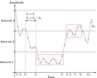
Fig. 1. A 3-state DTMC modeling of the process and a corre-sponding window is presented. Note that the sequence is from an under-lying signal, which is real valued and continuous; and possibly corrupted by an arbitrary (not necessarily Gaussian) and bounded additive noise. However, the noise is not illustrated in this figure for presentational clarity. The time series is anomalous due to the two short-term irregularities: (i) In the boxed region on the left, it has an abnormally too long waiting time at state 1; and (ii) on the right, it has abnormally too many state transitions.

in detecting the anomalous power consumption events of the Dutch research facility [25], the desired scale of the anoma-lies is 1-day, and since the sampling rate is 96-readings per day, the best choice for the window length in this example is

.

In this study, we concentrate on real valued signals that are continuous (in the mathematical sense with respect to the time: amplitude vs time), and possibly corrupted by an arbitrary (not necessarily Gaussian) and bounded additive noise, where we use Markov chains to model the data with quantized amplitudes at discrete times. The Markov assumption here does not actu-ally bring limitations about the assumed model and the gen-erality is due to the Wold’s Decomposition [42], which basi-cally states that any covariance-stationary stochastic process can be decomposed as the sum of the two terms: an auto-re-gressive (AR) process (or equivalently a moving average (MA) process) and a deterministic mean signal. However, a direct ex-ploitation of Wold’s Decomposition leads to an infinite Markov state space, which is practically infeasible [43]. Therefore, to reduce the number of states, we partition the amplitudes into levels, i.e., intervals. Note that although our model, i.e., the in-troduced birth-death type DTMC model, is a first order Markov model, the extension to higher orders is easily possible within our formulation by re-defining the history, i.e., concatenation, of sufficiently many previous states as the “new states” of a new and first order corresponding equivalent model. Regarding this straightforward extension, if one desires to use previous obser-vations, i.e., states, for a ’th order Markov chain, then she/he

would obtain a state space of cardinality with possibly a general Markov chain with almost arbitrary transitions between states violating our birth-death type chain assumption at the cost of increased computational complexity. Nevertheless, due to the almost negligible computational costs of the proposed algorithm for first order birth-death type Markov chain, one can comfort-ably use our algorithm at higher orders up to a certain level.

This quantization in amplitudes into levels through the in-troduced DTMC modeling can also serve as an effective dimen-sionality reduction or an effective feature extraction step -in ad-dition to the noise handling capabilities- with limited or no in-formation loss. Thus, this quantization technique can actually improve the learning rates of the model to be learned by re-ducing the number of parameters/dimensionality and hence by mitigating the overfitting issues. For instance, the authors of [3] quantize the pixel intensity readings in time into only levels for the proposed “statistical behaviour subtraction” [3]. Similarly, in terms of the Gaussian Mixtures Models (GMM) based background subtraction in video signals, is typically around 5 [44]. Hence, we consider that quantization in ampli-tude is, in general, not restrictive and this quantization level -as a design parameter- should actually be chosen as small as possible with respect to the target application while preserving information as much as possible. There is an obvious trade-off here: the assumed DTMC model might start losing from its modeling power as gets further smaller, and also cannot be arbitrarily large since then the noise tolerance of the assumed DTMC model decreases, i.e., it becomes more sensitive, as gets larger. Nevertheless, this trade-off can be easily avoided by straightforwardly extending from birth-death type of Markov chains to the general Markov chains that allow arbitrary tran-sitions between any states. Also, it is always possible to use a suitably smaller to obtain a birth-death type chain. For in-stance, the non-trivial choice of , which always yields a birth-death type chain, has been successfully applied to video anomaly identification [3].

Furthermore, the use of the birth-death type Markov chain in our study does not cause loss of generality because our formu-lations can be straightforwardly extended to cover the general setting of the Markov chains with arbitrary transitions between any states and remove the birth-death type Markov assumption. On the other hand, our focus in this study is to obtain, as the first time in the literature, the online implementation of the Neyman-Pearson (NP) characterization for the anomaly detection in time series data in a truly online manner with negligible computa-tional costs without requiring parameter tuning. To that end, as an initial study in this direction, we consider the birth-death type Markov chains, i.e., a special case of general Markov chains, that has been applied to the data with great success in a wide variety of signal processing and machine learning applications [3], [5]–[7], [44]–[49] ranging from the counting processes, e.g., queueing theory or population dynamics [45], as well as regres-sion/classification tasks [48], [49] to video anomaly identifica-tion [3].

In our approach, we consider the small variations of a signal at any state as insignificant variations, i.e., as contamina-tion/noise, and hence discard them. In this sense, we do not assume that the noise is negligible. Instead, we directly handle the noise either by discarding within state variations or by

allowing noisy transitions. Thus, we concentrate on the transi-tions (large variatransi-tions)/waiting times (persistency) between/at states. In fact, within state variations become increasingly minute as the number of the states/regions of the amplitude increases. For example, two different sequences

and mapping to the same state sequence , where is the state of the ’th observation in , are considered “same” up to small variations. In this sense, we can continue our derivations with only the state sequence without referring to the actual sequence . However, to emphasize the effect of the introduced DTMC as a mapping from to and the corresponding equivalence in between, we opt to use “ ” to refer to both the state sequence and the actual sequence simultaneously unless it is necessary to explicitly state the distinction. For example, is -to be more precise- the probability of the state sequence under the introduced DTMC model.

Based on this DTMC model, the density of a window from of finite length is given by, cf. [45],

where is the prior probability for the initial state that ac-counts for the initial conditions, is the waiting time for the window at the state observed right before the th transition,

i.e., , for , where is the time

of the last observation before the ’th transition with .

Also, with is the corresponding

se-quence of states observed before each transition. Note that the last transition is hypothetically assumed to be and is the total number of transitions, which can be as small as only 1 transition. If we accumulate a total waiting time at state as , then the log-likelihood is given by

(4) where is the total number of state observations

in with the exception that and

is the number of “up/right” (“down/left”) transitions

from state in , i.e., and

. Note that the log-likelihood expression in (4) is exact with the convention

when or to handle the boundary conditions.

Remark: We observe that a significant reduction via the

pro-posed observation model is possible with no or limited informa-tion loss. Since our DTMC model is a birth-death type Markov chain, the number of up and down transitions between two states must be (almost) equal due to the Global Balance (GB) equa-tions, i.e., . Therefore, the accumulated total waiting times ’s at each unique state as well as the corre-sponding number of transition occurrences provide suffi-cient statistics and are the only signal attributes to be necessarily stored. In this sense, is a complete set of de-scriptors of dimensionality that is independent of the length of the sequence .

We derive the log-likelihood density in the following Section III-B in order to later devise our anomaly detection methods in Section III-C.

B. The Log-Likelihood Density

In this part, we approximate the probability density of the log-likelihood in order to efficiently find the threshold of the anomaly detection test formulated in Section II. We start with concentrating on the random variables , i.e., and , in ; and then continue with for this derivation.

Let us define and

, in which and are the corresponding estimation errors. Then, we can write (4) as

(5) where is a constant with

and is an approximation term with

By ergodicity of the process and by weak law of large numbers (WLLN), , as the length of the sequence goes to infinity, i.e., as in probability. Furthermore, we point out that as is random, the log-likeli-hood is also random with the density , to which the initial condition has a negligible contribution for large . Conditioned on the knowledge of , since ( and ) are Maximum Likelihood (ML) estimators of the two parameters of a multinomial random variable (with three outcomes), they are unbiased with covariance and normally distributed for large , i.e.,

, where

We point out that ’s are correlated, which can be observed from the Global Balance (GB) equations from our birth-death type Markov chain, i.e., . Nevertheless, conditioned on the complete knowledge of ; we naively sup-pose that is also normally distributed for large with mean

, where (contribution of

the initial and termination conditions is neg-ligible for sufficiently long observations), is the transpose of

; and variance , where

(contribution of is negligible), i.e.,

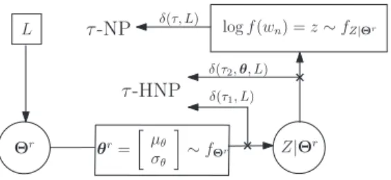
Fig. 2. The log-likelihood density model based on the mixture of Gaussians in (8). First the parameter is sampled from ; then, the log-likelihood is sampled from .

Similarly, the steady state probability can be approximated [50] by the estimator , which is unbiased with covariance , where

is the matrix of transition probabilities consisting of the terms , and with being the diagonal matrix of . For sufficiently large , is normally distributed,

i.e., and hence,

(7) Note that the density effectively defines a Gaussian prior on the mean and the variance of the conditional density . We can further obtain a reduced set of random

param-eters , where4 _{with the}

corresponding density .

As a result of this, we obtain

yielding to the (unconditional) log-likelihood density as (8) is a mixture of Gaussians, cf. Fig. 2.

As a final remark in this section, our derivations can be straightforwardly extended to the general Markov chain with arbitrary transitions between any states (not only between the neighboring states as in the birth-death type chain) at the cost of increased computational complexity. For this purpose, the log-likelihood in (4) is first updated to incorpo-rate the new probabilities s of such arbitrary transitions from state to state with with the corresponding number of observed transitions s. Then, the same func-tional log-likelihood form in (5) can be obtained with the new

variables defined as ,

, where is

similarly the corresponding error term. Therefore, all of the log-likelihood density derivations and the Gaussian approx-imations in our formulation remain valid and the rest of the derivations for the extension to the general Markov chain fol-lows similar lines. Hence, the corresponding reduced mixture of Gaussians form of (8) is straightforwardly derived in the same exact way to obtain our algorithm HNP as illustrated in Fig. 2 in the case of the general Markov chains.

4 _{is the transpose of a matrix .}

C. Anomaly Detection Methods

In this section, we propose two Neyman-Pearson (NP) test based anomaly detection methods that we compare in our experiments. A) An NP test with the threshold in (3) that is based on extensive Monte Carlo simulations named as “MCNP”. B) A hierarchical NP test based on the derived mixture of Gaussians form of the log-likelihood density, named as “HNP”, for which we also present a computationally highly efficient online algorithm without requiring Monte Carlo simu-lations or parameter tuning (“Sequential HNP”) in Section IV. Regardless of whether the source is stationary or non-stationary, the method HNP successfully achieves the desired false alarm rate while maximizing the detection power.

The proposed anomaly detection method HNP is a hierar-chical application of two successive NP tests: the first one uses the marginal density of and the second one uses the log-like-lihood density conditioned on , cf. Section III-C-2. During this hierarchical application, HNP allows one to analytically cal-culate the thresholds (of its two individual NP tests) as simple functional evaluations without requiring Monte Carlo simula-tions and complicated parameter tunings; and hence, yields a computationally highly efficient and online algorithm (Sequen-tial HNP in Section IV). On the contrary, the NP test in (3) is not analytically tractable. Namely, the threshold of the NP test cannot be determined analytically, i.e., Monte Carlo simulations are necessarily used in the MCNP method. Secondly, the overall detection rate of anomalies for the test method HNP is not the best achievable when the anomalies are uniformly distributed; however, it is preferable in our study due to its efficiency. Nev-ertheless, the individual tests in the HNP test are all separately the most powerful as they are NP tests and the resulting HNP test is uniformly the most powerful over the variable while achieving the desired false alarm rate . Moreover, when the anomalies are not uniformly distributed but appear as a change in the statistics of the underlying process , the optimality in the NP test is certainly lost and the proposed method HNP out-performs the method MCNP, cf. our experiments in Section V.

1) An NP Test Based on Extensive Monte Carlo Simulations (MCNP): In order to avoid the effects of the imperfect Gaussian

approximation in deriving the log-likelihood density when the window length is not sufficiently large, the first method we propose is an NP test, which is based on the exact form and the exact density of the likelihood in (4); however, it heavily relies on extensive Monte Carlo simulations. We em-phasize that this test is a generalization of the anomaly iden-tification method in [3] to multi state birth-death type Markov chains and serves as a comparison basis in our experiments. In-stead of approximating the density of and calcu-lating an approximate threshold for a specified false alarm rate , we estimate this threshold via extensive Monte Carlo simu-lations. In these simulations, we first randomly generate many samples of and obtain a set of realizations. Note that while generating a sample , we actually sample a sequence of a fixed and specified window length using the DTMC model and calculate via (4). Sup-pose that the set is sorted in the ascending order, i.e., for any , then we estimate the true threshold in (3) as , which precisely provides the anomaly detection method described in Section II.

Algorithm 1: Sequential HNP Input:

1:

2: while is sequentially streamed; and for do 3: via the update rule in (14)

4: via the rule in (13) using the window 5: Update the model parameters via the rule in (12) 6: 7: 8: if then 9: Declare anomaly at 10: else 11: 12: if then 13: Declare Anomaly at 14: end if 15: end if 16: end while

Return: All found anomalies

2) A Hierarchical NP Test (HNP): Based on the conditional

independency structure that is observed as a mixture of Gaus-sians in the final form of the log-likelihood density in (8), one can intuitively separate the anomaly detection problem into two pieces. Accordingly, we finally propose a hierarchical anomaly detection test method HNP that first applies an NP test for an anomaly against and -if not found an anomaly- secondly ap-plies an NP test for an anomaly against . We formulate this hierarchical test as

(9) In order to ensure an overall false alarm rate , we also require

the condition , where and are the false

alarm rates of the tests for and the conditional observation , respectively.

Unlike the MCNP method, the HNP method requires in ad-dition to the log-likelihood that is directly observable through from a window sequence of length to be tested. Then, we determine the threshold from

where is exponentially distributed with mean 2 since the ex-ponent of a bivariate Gaussian is chi-squared distributed with degree of freedom 2, and

is related to the normalization constant of a bivariate Gaussian. Hence, we obtain

(10) Similarly, we obtain

(11)

where is the cumulative distribution function for normal distribution. Finally, the overall false alarm budget is to be

shared between and such that is

satisfied to maximize the detection. This is a design issue and in

this work, we set .

We point out that the method HNP does not require Monte Carlo simulations even for varying window lengths and varying source statistics since the thresholds are derived analytically. This allows a sequential and computationally highly efficient anomaly detection algorithm, cf. Section IV.

3) Estimation of the Model Parameters: Both the proposed

methods MCNP and HNP require the knowledge of the model parameters and recall that in this study, we are presented a sequence and we would like to detect anoma-lous (sliding) windows in . To estimate these model parame-ters, we use another sliding estimation window with length

, where note that and includes .

Then, our model parameter estimators using the signal attributes extracted from are as follows:

(12) where we use the “ ” notation to refer to both cases respec-tively, i.e., we have two equations in (12) respectively for and . Although the steady state distribution can be an-alytically calculated by using the global balance equations for a birth-death type process, we also estimate it for the sake of completeness.

IV. SEQUENTIALHNP

We observe that the estimation of the model parameters, the evaluation of the log-likelihood expression in (4) and the calcu-lation of the HNP thresholds can all be sequentially performed through a simple update. Based on this observation, we present our sequential and computationally highly efficient algorithm for the proposed anomaly detection method HNP (Sequential HNP). In the following, we describe the details of the updates for parameter learning and log-likelihood calculations that are necessary in our sequential implementation.

Parameter Learning Updates: We need to develop

sequen-tial updates for the observation dependent variables in our parameter estimation equations in (12). Suppose that we have calculated based on the sequence

at time ; and let be the state of the

’th observation in the sequence . After reading the instance , we can update these variables as

(13) and as well as are similarly updated and we slide the parameter estimation window by one step.

Log-Likelihood Updates: Suppose that we have

, where , and we would like to calculate with an update over without a re-calculation after

reading the instance . Let be the state

of the ’th observation in the sequence , then it is straight-forward to show that

TABLE I

AVERAGEFALSEALARMRATESACHIEVED BY THEHNP METHODAPPLIED TO100 RANDOMLYINITIALIZEDMARKOVMODELSOVER5000 SEQUENCES PER

EACHMODEL FORVARYINGNUMBER OFSTATES , SEQUENCELENGTH ANDDESIREDRATES

and similarly for all of the other cases: i) and ; ii) and ; and iii) otherwise.

Based on these sequential likelihood and parameter updates in (13) and (14), as well as the threshold rules of HNP in (10) and (11), we present the sequential HNP in Algorithm 1.

Unlike the method MCNP, we analytically calculate the appropriate thresholds for a specified desired false alarm rate without using Monte Carlo simulations in our anomaly detection method HNP. This is a strong attribute of HNP that allows a generalization of our problem formulation to non-stationary sources with real time processing capabilities in a computationally highly efficient framework. Here, we assume “slow changes”, i.e., “continuous drifts over time”, in the source statistics to define the non-stationarity whereas an abrupt, i.e., sudden, change is used to define an anomaly, which differentiates non-stationarity from anomalies. Thus, anomaly detection in non-stationary environments is still reasonable and an effective tool. Note that the “slow” change in the source sta-tistics refers to the “slow” rate of drift in the model parameters learned for the discrete signal obtained after the sampling of the underlying non-stationary continuous signal.

Consider a data stream from a non-stationary stochastic process such that its statistical properties change slowly in time; and we sequentially detect the anomalous windows of length in in real time. Our approach is to sequentially learn the time-varying model parameters in a wider and sliding

window with and using the

es-timation equations in (12) and the corresponding update rules in (13), which provides the real-time adaptation to non-station-arity. Meanwhile, we apply our test at every time for windows

of length , with and , using

the HNP decision rule in (9) and the corresponding updates in (14). The complete algorithmic description is provided in Algo-rithm 1. Since our method requires only basic function evalu-ations and a few simple operevalu-ations such as additions and sub-tractions, our method can be applied to stationary or non-sta-tionary data streams with performance guarantees, i.e., NP op-timality, at negligible computational costs without parameter tuning and without a re-training phase and even sequentially in a truly online manner. On the other hand, the method MCNP or the well-known other methods in the literature such as the nearest neighbor graph based detections continuously require a re-training phase, which makes them non-applicable (if one de-sires to maintain the crucial NP optimality) when the source is non-stationary.

Our purpose in parameter estimation in non-stationary envi-ronments is to capture, i.e., learn, an average behaviour of the time varying characteristics in the signal due to the non-station-arity, where the precise inference at each time is not reasonable, if not impossible. In order for the parameter estimation under non-stationarity to be reasonable, the variation in the model pa-rameters, i.e., change in the source statistics, should be “slow” so that a meaningful average behaviour can be extracted and a test for an anomaly against the extracted average behaviour can be performed. Otherwise, if the non-stationarity in the signal is chaotic, then no such average behavior can be extracted and the problem itself becomes technically trivial; although the detection becomes more difficult. if the non-stationarity is chaotic, then one can observe every sequence with no surprize; and hence, one can readily use a nominal model (without a need for parameter estimation or learning) with parameters such that all possible sequences are of the same probability.

V. EXPERIMENTS

In our first set of experiments, we concentrate on the achiev-ability of the specified false alarm rate. Note that the MCNP test method can achieve this rate arbitrarily accurately with exten-sive simulations. However, the proposed test HNP is designed to match the desired rate without such simulations. To this end, we devise experiments with the number of states

and the sequence length for varying desired

false alarm rates . For

a given , and as well as a set of randomly chosen model parameters, i.e., , we generate 5000 length-(normal) sequences directly from the Markov model and count the number of anomaly decisions (by HNP) that yields a false alarm rate. We report the achieved average false alarm rates over 100 randomly initialized model parameters in Table I.

We observe that the proposed method HNP approximates the desired false alarm rate more accurately for longer sequences since the Gaussianity assumption for the estimation error of the multinomial parameters also improves with the sequence length. Similarly, since the inter-state dependencies decrease as the number of states increases, we obtain a better achiev-ability for relatively larger ’s. Finally, the proposed method HNP achieves the desired false alarm rate in most of the cases with 1% error with the sequences of length or longer. We next compare the MCNP test method with the HNP test method in terms of the Receiver Operating Characteristics (ROC). In these comparisons, we concentrate on two types

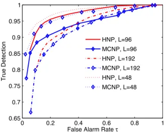
Fig. 3. The HNP test method significantly outperforms the MCNP test method when the anomalies are in terms of the abrupt model changes (cf. or

). On the other hand, when the anomalies are uniformly distributed, both methods perform comparably (cf. ).

of anomalies that are both due to a sudden change in the source statistics. In the case of the first type of anomalies, the anomalous sequences are still assumed to be drawn from a Markov model, however, whose parameters and the nominal model parameters are different. On the contrary, in the second type, anomalies do not necessarily follow a specific Markov model, where the anomalies are assumed to be uniformly and equally likely distributed in the observation domain. In this case, our purpose is to demonstrate the NP optimality since the described MCNP test is theoretically known to be optimal when the anomalies are uniformly distributed. To this end, we generate 5000 anomalous sequences of length , each of which is generated with respect to a randomly chosen different set of model parameters, whereas another set of 5000 normal sequences is generated with respect to a same and fixed nominal set of model parameters. In Fig. 3, we report the average ROC rates over 100 trials for varying number of states and desired rates . Secondly, we follow the same procedure, however; generate the anomalous sequences “truly uniformly” for the case . We observe that if the anomalies emerge as a change in the model parameters, then the proposed method HNP detects such anomalies at significantly higher rates compared to the method MCNP. Remarkably, NP optimality is observable only when the anomalies are truly uniformly distributed, cf. in Fig. 3.

We emphasize that the MCNP test method heavily relies on Monte Carlo simulations to achieve the desired false alarm rate, which is prohibitively complex for real time applications. On the contrary, the proposed HNP test method is compu-tationally highly efficient with almost negligible costs since it does not require such Monte Carlo simulations. This is a strong attribute of the HNP method, which makes it especially attractive when one needs to process non-stationary sources. We next concentrate on the truly sequential implementation of the proposed HNP method, where we perform experiments with non-stationary sources. In this part, we generate a se-quence of length that is specially exposed

Fig. 4. The HNP test method significantly outperforms the MCNP method at almost negligible computational costs when the signal source is non-stationary.

to drifting source statistics such that each instance is pro-duced based on the Markov model with the time varying

parameters of with , where

, . Hence,

the non-stationary data in this example is generated by simu-lating a relatively slow change from the Markov model with the transition matrix to the one with the transition matrix . We would like to detect the anomalous subsequences of of length using a sliding window approach, where we use wider sliding windows of length for estimating the active set of source statistics. We explicitly inject anomalies in by overwriting the first instances starting from every ’th instance of by the values uniformly drawn from the support set {1,2}. We also generate a label sequence , where indicates an anomaly such that the window includes more than anomalous points; and otherwise, . We run the proposed sequential HNP on randomly generated 10 different sequences and report the average ROC curves in Fig. 4. On the other hand, since the signal source in this experiment is non-stationary, the threshold for the MCNP test has to be calculated at every instance via Monte Carlo simulations, which is clearly practically infeasible. Instead, for the MCNP test, we estimate the threshold only once using the complete sequence . We observe that the proposed HNP test method significantly outperforms the MCNP test at almost negligible computational costs with non-stationary data. Next, we present our real data experiments, where we run our sequential HNP algorithm on the time series consisting of the power consumption readings of a Dutch research facility throughout the year 1997 [25]. These readings, i.e., power con-sumption measurements in 1997, are real and obtained every 15 minutes, which produces a sequence of length

(96 readings per day). In this experiment, we use intervals in the magnitude (the complete magnitude interval is [614,2152]) corresponding to low-[614, 1200), mid-[1200, 1600) and high-[1600, 2152] levels of power consumption. All of the choices of result in a birth-death type process as desired, however, we use since it is found to be appropriate by inspection. Since this data set is provided without a ground-truth for anomalies, we inject anomalies into

Fig. 5. Real data experiments on the power consumption data set. Our tech-nique HNP is also robust to the mismatches between the true scale of anomalies and the guessed scale.

the data set after the quantization in order to compare (using the ROC curve) the sequential HNP (our method) and the stan-dard NP test, i.e., MCNP, that is based on extensive Monte Carlo simulations. We inject anomalies as follows: During the first day of each month starting from February, we randomly over-write the power consumption data (after quantization) such that a random transition from a state to another possible one (in an equally likely fashion) is applied at any time during that day. This generates anomalous time instances in

total. We use (1 month) and

to also evaluate for possible mismatches between the true scale of anomalies (96 in this case) and the guessed scale ( in this case). We also use a label sequence corresponding to this se-quence of power readings such that in this label sese-quence, any time is labeled as anomalous if the test window ending at that time has more than 50% injected anomaly instances; and labeled as nominal, otherwise. Since it is computationally prohibitive to repeatedly perform Monte Carlo simulations at every time for the method MCNP, we perform those simulations only once (for the complete stream) to calculate the desired thresholds.

Then, based on this experimental setup, we plot the ROC curve in Fig. 5 reporting the true detection rates vs false alarm rates for the methods HNP and MCNP for all cases of (over 10 trials for injected random anomalies). We observe that our technique significantly outperforms the method MCNP in all cases due the non-stationarities in the power consumption data (for instance: months including holidays such as Good Friday or Christmas Eve consumes less power creating non-stationarity), to which the method MCNP cannot adapt (due to its computa-tional costs), whereas our online technique HNP demonstrates excellent adaptation due to its efficient design with controllable false alarm rate. Finally, we also observe that our technique is also robust to the possible mismatches between the true scale of anomalies and the guessed scale.

VI. CONCLUSION

We introduce an online anomaly detection algorithm for tem-poral data under practical real life constraints to specifically ad-dress the contemporary applications requiring sequential data processing at large scales/high rates. The proposed algorithm is

computationally highly efficient such that data streams at ex-tremely fast rates can be processed in real time. Our algorithm also allows real time controllability of the Type-I error, i.e., false alarm rate, by nearly achieving a user specified false alarm rate while maximizing the detection power regardless of whether the source is stationary or non-stationary. Moreover, we do not re-quire parameter tuning (to match the desired rates) even if the source statistics change. The proposed algorithm sequentially learns the possibly varying nominal Markov statistics in a time series and detects the anomalous, i.e., statistically sufficiently deviant, subsequences based on a Neyman-Pearson (NP) char-acterization for anomalies. The presented study is highly novel since we are the first to provide an online NP solution to the problem such that the NP optimality, i.e., maximum detection power at a specified false alarm rate, is nearly achieved in a truly online manner.

REFERENCES

[1] H. Wang, M. Tang, Y. Park, and C. Priebe, “Locality statistics for anomaly detection in time series of graphs,” IEEE Trans. Signal

Process., vol. 62, no. 3, pp. 703–717, 2014.

[2] M. Filippone and G. Sanguinetti, “A perturbative approach to novelty detection in autoregressive models,” IEEE Trans. Signal Process., vol. 59, no. 3, pp. 1027–1036, 2011.

[3] V. Saligrama, J. Konrad, and P. Jodoin, “Video anomaly identifica-tion,” IEEE Signal Process. Mag., vol. 27, no. 5, pp. 18–33, 2010. [4] J. Lehtomaki, J. Vartiainen, M. Juntti, and H. Saarnisaari, “Cfar outlier

detection with forward methods,” IEEE Trans. Signal Process., vol. 55, no. 9, pp. 4702–4706, 2007.

[5] V. Chandola, A. Banerjee, and V. Kumar, “Anomaly detection: A survey,” ACM Comput. Surv. (CSUR), vol. 41, no. 3, p. 15, 2009. [6] V. Chandola, A. Banerjee, and V. Kumar, “Anomaly detection for

dis-crete sequences: A survey,” IEEE Trans. Knowl. Data Eng., vol. 24, no. 5, pp. 823–839, 2012.

[7] M. Gupta, J. Gao, C. Aggarwal, and J. Han, “Outlier detection for tem-poral data: A survey,” IEEE Trans. Knowl. Data Eng., vol. 26, no. 9, pp. 2250–2267, 2014.

[8] S. Rajasegarar, C. Leckie, and M. Palaniswami, “Anomaly detection in wireless sensor networks,” IEEE Wireless Commun., vol. 15, no. 4, pp. 34–40, 2008.

[9] V. Saligrama and M. Zhao, “Local anomaly detection,” in Proc.Int.

Conf. Artif. Intell. Statist., 2012, pp. 969–983.

[10] H. Ozkan, O. Pelvan, and S. Kozat, “Data imputation through the iden-tification of local anomalies,” IEEE Trans. Neural Netw. Learn. Syst., vol. PP, no. 99, p. 1-1, 2015.

[11] V. Poor, An Introduction to Signal Detection and Estimation. New York, NJ, USA: Springer Sci. Bus. Media, 1994.

[12] V. Jumutc and J. Suykens, “Multi-class supervised novelty detec-tion,” IEEE Trans. Pattern Anal. Mach. Intell., vol. 36, no. 12, pp. 2510–2523, 2014.

[13] X. Ding, Y. Li, A. Belatreche, and L. Maguire, “Novelty detection using level set methods,” IEEE Trans. Neural Netw. Learn. Syst., vol. 26, no. 3, pp. 576–588, 2015.

[14] Y. Chen, X. Dang, H. Peng, H. Bart, and H. Bart, “Outlier detection with the kernelized spatial depth function,” IEEE Trans. Pattern Anal.

Mach. Intell., vol. 31, no. 2, pp. 288–305, 2009.

[15] H. Ferdowsi, S. Jagannathan, and M. Zawodniok, “An online outlier identification and removal scheme for improving fault detection per-formance,” IEEE Trans. Neural Netw. Learn. Syst., vol. 25, no. 5, pp. 908–919, 2014.

[16] B. Schölkopf, J. Platt, J. Shawe-Taylor, A. Smola, and R. Williamson, “Estimating the support of a high-dimensional distribution,” Neural

Computat., vol. 13, no. 7, pp. 1443–1471, 2001.

[17] B. Liu, Y. Xiao, P. Yu, L. Cao, Y. Zhang, and Z. Hao, “Uncertain one-class learning and concept summarization learning on uncertain data streams,” IEEE Trans. Knowl. Data Eng., vol. 26, no. 2, pp. 468–484, 2014.

[18] C. Manikopoulos and S. Papavassiliou, “Network intrusion and fault detection: A statistical anomaly approach,” IEEE Commun. Mag., vol. 40, no. 10, pp. 76–82, 2002.

[19] C. Scott and R. Nowak, “Learning minimum volume sets,” J. Mach.

Learn. Res., vol. 7, pp. 665–704, 2006.

[20] M. Zhao and V. Saligrama, “Anomaly detection with score functions based on nearest neighbor graphs,” Adv. Neural Inf. Process. Syst., pp. 2250–2258, 2009.

[21] M. Basseville and I. Nikiforov et al., Detection of Abrupt Changes:

Theory and Application. Englewood Cliffs, NJ, USA: Prentice-Hall,

1993, vol. 104.

[22] K. Zhang, M. Hutter, and H. Jin, “A new local distance-based outlier detection approach for scattered real-world data,” Adv. Knowl. Discov.

Data Mining, pp. 813–822, 2009.

[23] S. Ramaswamy, R. Rastogi, and K. Shim, “Efficient algorithms for mining outliers from large data sets,” ACM SIGMOD Rec., vol. 29, no. 2, pp. 427–438, 2000.

[24] A. Hero, “Geometric entropy minimization (gem) for anomaly detec-tion and localizadetec-tion,” Adv. Neural Inf. Process. Syst., pp. 585–592, 2006.

[25] E. Keogh, J. Lin, S. Lee, and H. Van Herle, “Finding the most un-usual time series subsequence: Algorithms and applications,” Knowl.

Inf. Syst., vol. 11, no. 1, pp. 1–27, 2007.

[26] E. Keogh, J. Lin, and A. Fu, “Hot sax: Efficiently finding the most un-usual time series subsequence,” in Proc. IEEE Int. Conf. Data Mining, 2005.

[27] L. Wei, E. Keogh, and X. Xi, “Saxually explicit images: Finding un-usual shapes,” in Proc. Int. Conf. Data Mining, 2006, pp. 711–720. [28] Y. Bu, O. Leung, A. Fu, E. Keogh, J. Pei, and S. Meshkin, “Wat:

Finding top-k discords in time series database,” in SDM, 2007, pp. 449–454.

[29] A. Fu, O. Leung, E. Keogh, and J. Lin, “Finding time series discords based on Haar transform,” Adv. Data Mining Appl., pp. 31–41, 2006. [30] J. Lin, E. Keogh, A. Fu, and H. Van Herle, “Approximations to magic:

Finding unusual medical time series,” in Proc. IEEE Symp.

Comput.-Based Med. Syst., 2005, pp. 329–334.

[31] E. Keogh, S. Lonardi, and C. Ratanamahatana, “Towards parameter-free data mining,” in Proc. Int. Conf. Knowl. Discov. Data Mining, 2004, pp. 206–215.

[32] D. Yankov, E. Keogh, and U. Rebbapragada, “Disk aware discord dis-covery: Finding unusual time series in terabyte sized datasets,” Knowl.

Inf. Syst., vol. 17, no. 2, pp. 241–262, 2008.

[33] X. Chen and Y. Zhan, “Multi-scale anomaly detection algorithm based on infrequent pattern of time series,” J. Computat. Appl. Math., vol. 214, no. 1, pp. 227–237, 2008.

[34] C. Shahabi, X. Tian, and W. Zhao, “Tsa-tree: A wavelet-based ap-proach to improve the efficiency of multi-level surprise and trend queries on time-series data,” in Proc. Int. Conf. Scientif. Statist.

Database Manage., 2000, pp. 55–68.

[35] L. Wei, N. Kumar, V. Lolla, E. Keogh, S. Lonardi, and R. Chotirat, “Assumption-free anomaly detection in time series,” SSDBM, vol. 5, pp. 237–242, 2005.

[36] Y. Zhu and D. Shasha, “Efficient elastic burst detection in data streams,” in Proc. Int. Conf. Knowl. Discov. Data Mining, 2003, pp. 336–345. [37] H. Ozkan, A. Akman, and S. Kozat, “A novel and robust parameter

training approach for HMMS under noisy and partial access to states,”

Signal Process., vol. 94, pp. 490–497, 2014.

[38] N. Ye et al., “A Markov chain model of temporal behavior for anomaly detection,” in Proc. IEEE Syst., Man, Cybern. Inf. Assur. Secur.

Work-shop, 2000, vol. 166, p. 169.

[39] C. Michael and A. Ghosh, “Two state-based approaches to program-based anomaly detection,” in Proc. Ann. Conf. Comp. Secur. Appl., 2000, pp. 21–30.

[40] V. Chandola, V. Mithal, and V. Kumar, “Comparative evaluation of anomaly detection techniques for sequence data,” in Proc. Int. Conf.

Data Mining, 2008, pp. 743–748.

[41] C. Marceau, “Characterizing the behavior of a program using multiple-length n-grams,” in Proc. 2000 Workshop on New Secur. Paradigms, 2001, pp. 101–110.

[42] J. Hamilton, Time Series Analysis. Princeton, NJ, USA: Princeton Univ. Press, 1994, vol. 2.

[43] B. Geiger, T. Petrov, G. Kubin, and H. Koeppl, “Optimal Kullback-Leibler aggregation via information bottleneck,” IEEE Trans. Autom.

Control, vol. 60, no. 4, pp. 1010–1022, 2015.

[44] Z. Zivkovic, “Improved adaptive Gaussian mixture model for back-ground subtraction,” in Proc. IEEE 17th Int. Conf. Pattern Recogn.

(ICPR), 2004, vol. 2, pp. 28–31.

[45] S. Karlin, A First Course in Stochastic Processes. New York, NY, USA: Academic, 2014.

[46] B. Moser and T. Natschlager, “On stability of distance measures for event sequences induced by level-crossing sampling,” IEEE Trans.

Signal Process., vol. 62, no. 8, pp. 1987–1999, 2014.

[47] D. Morgan, “On level-crossing excursions of Gaussian low-pass random processes,” IEEE Trans. Signal Process., vol. 55, no. 7, pp. 3623–3632, 2007.

[48] S. Kozat, A. Singer, and G. Zeitler, “Universal piecewise linear pre-diction via context trees,” IEEE Trans. Signal Process., vol. 55, no. 7, pp. 3730–3745, 2007.

[49] N. Vanli and S. Kozat, “A comprehensive approach to universal piece-wise nonlinear regression based on trees,” IEEE Trans. Signal Process., vol. 62, no. 20, pp. 5471–5486, Oct. 2014.

[50] M. Xue and S. Roy, “Spectral and graph-theoretic bounds on steady-state-probability estimation performance for an ergodic Markov chain,” in Amer. Contr. Conf., 2011, pp. 2399–2404.

Huseyin Ozkan received the B.Sc. degrees in electrical and electronics engineering, and mathe-matics from Bogazici University, Istanbul, Turkey, in 2007. He received the M.Sc. degree in electrical engineering from Boston University, MA, USA, in 2010; and the Ph.D. degree in electrical and electronics engineering from Bilkent University, Ankara, Turkey, in 2015.

He is also with the UGES Division at Aselsan Inc., Ankara, Turkey, where he conducts computer vision research for large are surveillance. Before joining Aselsan, he focused on anomaly detection and recommendation problems as a researcher at Turk Telekom Inc., Ankara. He also worked as a research intern at Mitsubishi Electric Research Laboratories, Cambridge, MA, USA, where he developed efficient algorithms for vision based road sign detection. His research interests include statistical learning, pattern recognition, computer vision and statistical signal processing.

Dr. Ozkan has been awarded the Best Paper award by the IEEE Conference on Advanced Video and Signal-based Surveillance (2011); and the Best Student Paper award by the IEEE Conference on Signal Processing Applications (2012).

Fatih Ozkan received the B.Sc. degree in computer engineering from Cukurova University, Adana, Turkey, in 2012.

He is currently working toward the M.Sc. degree in the Department of Information Systems, Middle East Technical University. His research interests include computer vision and machine learning. He is also working as a full-time researcher in the ILTAREN Institute at TUBITAK, Ankara, Turkey.

Suleyman S. Kozat (SM’12) received the B.Sc. de-gree in electrical and electronics engineering from Bilkent University, Ankara, Turkey. He received the M.S. and Ph.D. degrees in electrical engineering from the University of Illinois at Urbana Champaign, IL, USA, in 2001 and 2004, respectively.

After graduation, he joined IBM Research, T. J. Watson Research Center, Yorktown, NY, USA, as a Research Staff Member in Pervasive Speech Technologies Group, where he focused on problems related to statistical signal processing and machine learning. He also worked as a Research Associate at Microsoft Research, Redmond, WA, USA, in Cryptography and Anti-Piracy Group. Currently, he is an Associate Professor with the Electrical and Electronics Engineering Department, Bilkent University, Turkey. His research interests include intelli-gent systems, adaptive filtering for smart data analytics, online learning, and machine learning algorithms for signal processing.

Dr. Kozat has been awarded the IBM Faculty Award by IBM Research in 2011, Outstanding Faculty Award by Koc University in 2011, Outstanding Young Researcher Award by the Turkish National Academy of Sciences in 2010, ODTU Prof. Dr. Mustafa N. Parlar Research Encouragement Award in 2011, and holds the Career Award by the Scientific Research Council of Turkey, 2009.