The permutation flow shop problem with sum-of-completion times performance criterion

Completion Times Performance Criterion

Selcuk Karabati

Management Department, Faculty of Business Administration, Bilkent University, 06533 Bilkent, Ankara, Turkey

Panagiotis Kouvelis

The Fuqua School of Business, Duke University, Durham, North Carolina, 27706

In this article we address the non-preemptive flow shop scheduling problem for minimization of the sum of the completion times. We present a new modeling framework and give a novel game-theoretic interpretation of the scheduling prob- lem. A lower-bound generation scheme is developed by solving appropriately de- fined linear assignment problems. This scheme can also be used as a heuristic approach for the solution of the problem with satisfactory results. Its main use, however, is as a bounding scheme within a branch-and-bound procedure. O u r branch-and-bound procedure improves significantly upon the best available enu- merative procedures in the current literature. Extensive computational results are used to qualify the above statements. 0 1993 John Wiley & Sons, Inc.

1. INTRODUCTION

We address the non-preemptive permutation flow shop scheduling problem with the sum of completion times as the performance criterion. The above problem can be stated as follows. Each of the n jobs, J , , J 2 ,

. . . ,

I,,,

has to be processed on m machines, M I , M 2 ,

. . .

, M,, in that order. The processing of job J , on machine M, requires an uninterrupted period of processing time p , . , . Each machine can process at most one job at a time. The objective is to find a permutation schedule, i.e., a single ordering of the jobs on all machines, such that the sum of completion times is minimized. Minimizing the sum of completion times amounts to minimizing the mean completion time of jobs as well. A permutation schedule is represented by a = (a(l), a(2),

. . . , a ( n ) ) ,

where

a(i) is the ith job in the processing order. In our further discussion when we refer to a schedule a w e mean a permutation schedule, unless specified otherwise. Because the problem is NP-hard for m L 2 (see Gonzalez and Sahni [6]), enumerative and/or heuristic approaches are essentially unavoidable. For m =

2, solution procedures have been developed by Ignall and Schrage [7] and Kohler and Steiglitz [8]. A lower bounding scheme for m = 2 was proposed by Ignall

Naval Research Logistics, Vol. 40, pp. 843-862 (1993)

844 Naval Research Logistics, Vol. 40 (1993)

and Schrage [7]. Their procedure was generalized to arbitrary m by Bansal [3]. Ahmadi and Bagchi [ 11 improved upon Bansal’s bounding scheme. Miyazaki, Nishiyama, and Hashimoto

[

111, and Szwarc

[

151 have developed sufficient op- timality conditions for the problem using a pairwise interchange method. Mi- yazaki et al. [ l l ] presented also a heuristic solution procedure.

In this article we expand on the modeling framework of Monma and Rinnooy Kan

[

121 for permutation flow shops. We model the problem as a two-person zero-sum game. Using this new modeling approach, we present a lower-bounding scheme that requires the solution of a series of linear assignment problems. Using this bounding scheme and a new branching approach, we develop an efficient branch-and-bound procedure for the problem. The main ideas of our bounding scheme can also be used to generate a good heuristic solution to the problem.

The structure of the article is as follows. In Section 2 we present our modeling framework and discuss a class of linear assignment problems which will play an important role in the rest of the article. A novel interpretation of the flow shop scheduling problem in a game theoretic context is presented in Section 3. In Section 4 we discuss a new lower-bound generation approach based on the results of Sections 2 and 3. Capitalizing on the results of Section 4, we develop a new branch-and-bound scheme for permutation flow shops in Section 5 . We report on our computational experience with this new approach in Section 6. Finally, Section 7 summarizes our results and discusses some potential extensions of our modeling approach.

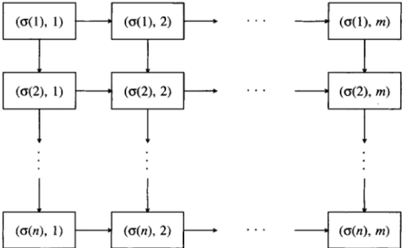
2. CRITICAL PATHS, ASSIGNMENT PROBLEMS, AND THE PERMUTATION FLOW SHOP SCHEDULING PROBLEM For a schedule w we can define a recursive relationship to find the completion time C<,(,),, of job I,,,,) on machine M , as follows (for detailed explanations refer to Baker [2] and Monma and Rinnooy Kan [12]):

where Co(o)., = Co(,).o = 0. The recursive structure (1) can be equivalently presented, as pointed out by Monma and Rinnooy Kan [12], by the directed graph G depicted in Figure 1. Vertices (cr(i), j ) are defined for each element o(i) of the permutation and each machine M,. A weight po,,),, is associated with vertex ( ( ~ ( i ) , j ) . Directed arcs are defined from each vertex ( a ( i ) , j ) toward (a(i

+

l ) , j ) and (w(i), j

+

1).

Given the above-defined graph G, the completion time

Co,,),,

of job .I,,,,,, on machine M , , in the permutation schedule w, is equal to the maximum-weighted

directed path from (w(l), 1) to (a(i), j ) in the graph. Therefore, the sum of completion times of jobs in schedule w, F ( a ) , is given by

Any path from ( a ( l ) , 1) to ( ( ~ ( i ) , m ) which attains the value Crr(i).nl is called a

&&+

. . '

+A,

Figure 1. Directed graph ( G ) representation of a permutation schedule u.

the sum of completion times of a schedule is analogous to the determination of n maximum paths, one for each job, on an acyclic graph with positive arc lengths. The computational complexity of determining all such paths is O(nm) (Lawler Let T ( i ) be a path from ( ~ ( l ) , 1) to ( a ( i ) , m ) on the directed graph G. Szwarc

[15] makes the observation that the length f ( a ( i ) , T ( i ) ) of the path T ( i ) can be

presented as [lo]).

where 1 5 t(i, 1) 5 t(i, 2) 5

...

5 t(i,

i

- 1) 9 m are appropriate integers which uniquely define ~ ( i ) . Let denote the set of all such paths on the direct graph G for job .I,,,,). Then F ( a ) , the sum of completion times, can be rewritten as

By letting T =

T , we can rewrite ( 3 ) as

x T2.n, x

...

x T,,nl, and T = ( ~ ( l ) , 7 ( 2 ) , .

.

. ; ~ ( n ) ) E

Then, if S,, is the set of all permutation schedules, the permutation flow shop scheduling problem for minimization of the sum of completion times can be formulated as follows:

846 Naval Research Logistics, Vol. 40 (1993)

Using the above established modeling framework, we can now state the following proposition. For presentation convenience, we use the usual abbreviation nlml PIC. Ci for the n-job m-machine permutation flow shop scheduling problem with

the sum-of-completion-times performance criterion. PROPOSITION 1:

holds:

max min YET u€S,,

For the nlmlPIC Ci problem the following relationship

I1 n

PROOF: Let a. E

Sn

be a specific permutation schedule and E T be a path vector on the directed graph G. Then

n n N

However, (7) holds for every no E S,, and T , ~ E T , therefore the validity of (6)

follows immediately.

0

Let F ( a , T ) = E:=, f(a(i), T(i)), a E

Sn

and T E T. Then Proposition 1 states that for any path vector T E T , the solution to the optimization problem

( A P ) : min F ( a , T )

U€ s,,

provides a lower bound for the problem as formulated in ( 5 ) . Some further insight on the nature of ( A P ) is provided by the following result.

PROPOSITION 2: ( A P ) is equivalent to a linear assignment problem. PROOF: According to (2), for a specific path T ( i ) in path vector 7 E T ,

there exists a unique set of integers (t (i, l ) , t(i, 2 ) ,

.

.

. , t(i, i

- 1 ) ) such that for any a E S,, we have the following:

where 1{.} is an indicator function and the integers t(i, 0) and t(i, i ) assume the values 1 and m, respectively. Note that we have 1 5 t(i, 1 ) 5 t(i, 2 ) 5

...

5 t(i,

i - 1 ) I m. Now by letting t(i, k ) = 0 , i

<

k 5 n we can rewrite (8) as

~ r = l ] = I k = t ( i , j - l )

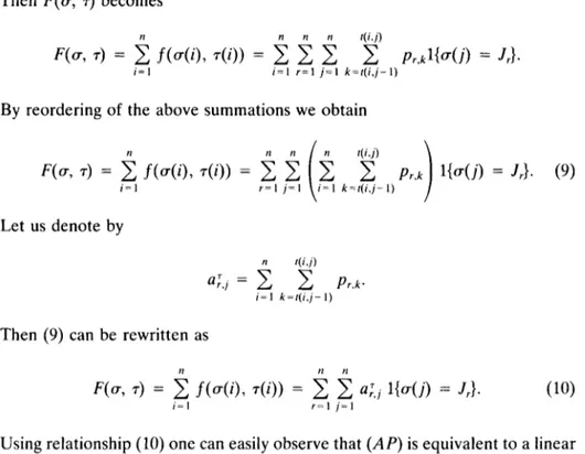
Then F ( a , T ) becomes

By reordering of the above summations we obtain

Let us denote by

Then (9) can be rewritten as

Using relationship (10) one can easily observe that ( A P ) is equivalent to a linear assignment problem with cost matrix A' = (u;,!).

0

EXAMPLE: We now present a numerical illustration of Proposition 2. Con- sider a three-job, two-machine problem with the paths given in Figure 2. For these paths we have the following path weights:

Machines 1 Position 2 3 1 2

E

848 Naval Research Logistics, Vol. 40 (1993) We also have

Now using this relationship we can show that min, F ( a , 7) is a linear assignment

problem with the following assignment matrix:

Location

Job 1 2 3

Using Proposition 1, we can easily state a sufficient condition for the optimality of a schedule v E S , .

PROPOSITION 3: Let a,) be a schedule in S,,, and T" be the path vector f o r

which F ( q , T") = maxTETF(a,,, T ) . ff F ( q , 7") = min,Ly,, F ( a , T"), then q l is an optimal schedule.

PROOF: From Proposition 1 we know that minOEs,, F ( a , T*) is a lower bound for the problem. From the statement of the proposition we have

F(a,,, T*) = max F(a,), T) = min F ( a , 7").

r E T UtS,,

Therefore, a,, is an optimal schedule.

0

Proposition 3 can be useful for the class of scheduling problems for which (6) holds as an equality. Our discussion below identifies such a class of problems in ordered flow shops and demonstrates how our modeling framework can be applied to derive one of the known results in the ordered flow shop literature (see Panwalkar and Khan [14]).

DEFINITION 1: A pow-shop problem is ordered if the following constraints are satisfied:

1. p,., > pk.1, for jobs i and k , and for some machine t, also implies p,,j 2 pk.,, j = 1,

. . . , m,

2. p,., p ,.,, for machines j and I, and for some job r, also implies P , , ~ 2 p ,,,, i = 1, . . . > n .

PROPOSITION 4: Consider the ordered flow shop problem. ff the largest processing time of each j o b is on the first machine, then the n l m l P l X C j problem

belongs to the special class of scheduling problems f o r which relationship (6) holds

as an equality. The S P T (shortest processing time) sequencing rule provides the optimal solution to the above ordered flow shop problem.

PROOF: Using results from Panwalkar and Khan [14], we can write the critical path vector T* = ( T * ( i ) ,

i

= 1,

.

.

. ,

n ) of the optimal schedule aspT in the following form:

Let us now consider the corresponding linear assignment problem for T*: ( A P ) : min F ( a , T * ) .

UES,,

The entries to the assignment matrix A" = (u;:]) are given by

l?l

u;., = ( n

+

1 - j ) p , , ,

+

C

pr,;, r = 1, . . . , n ; j = 1, . . . , n .

;=1

Note that the second term of a;:! is independent of j . Therefore the optimal solution to ( A P ) sequences the jobs in the SPT order, based on their processing times on Machine 1. Then, we have that for the resulting schedule the following relationship holds:

min F ( a , T*) = F ( q S p T , T * ) = max F ( a s p r , T ) .

W t S , , TE T

The last equality in the above relationship holds by the definition of T* as the

critical path vector for aSpT. Therefore, relationship (6) holds as an equal-

ity.

0

3. GAME-THEORETIC INTERPRETATION OF THE

nlmlPII:

C i

PROBLEM

The results of Section 2 point out the min-max nature of the nlrn/PIC C, problem. A problem with a similar min-max formulation has appeared in very different context, that of game theory. This fact motivated us to provide a game- theoretic interpretation of the n / r n / P / C C j problem. We will use this interpre- tation to directly apply an integer programming formulation of the corresponding game-theoretic problem to formulate our sequencing problem.

We may relate the formulation ( 5 ) of permutation flow shop problems to a two-person zero-sum game. Player 1, referred to as the path maker, has a pure strategy set T (set of path vectors) and Player 2, referred to as the schedule maker, has a pure strategy set S,l. For Player 1 the payoff of the game for pure strategies a E S,, and T E T is F ( a , T ) . Similarly, the loss of Player 2 is F(v, T ) .

In a two-person zero-sum game, there exists a pure strategy for player 1 by which he is certain to obtain at least a payoff of f , which is given by

f = max min F ( a , T ) . i € T rrES,,

-

850 Naval Research Logistics, Vol. 40 (1993)

the least loss independently of the actions of the path maker. The minimal loss for the schedule maker is given by

7,

where

7

= min max F ( P , T).

UES,! r E T

Observe that

7

is the optimal solution of the permutation flow shop problem. From the results of game theory (von Neumann and Morgenstern [18], we can immediately conclude that f 5

7,

an indirect verification of Proposition 1. In

case the sufficient conditionstated in Proposition 3 holds, i.e., f - = we say that the game has a saddle or equilibrium point.

The n / m / P / C C j problem can also be analyzed as a majorant game. In such a game the schedule maker makes his move and then the path maker chooses his strategy in full knowledge of the other player's move. It can be seen that the equilibrium point of the majorant game is given by

f * = min max F(w, T),

v€S,, r E T

and is equal to the optimal solution of the n l m l PIC C, problem. The equilibrium value of the majorant game, and as a consequence the solution to the n l m l P l

2

C, problem, can be found by solving the following integer programming

formulation:

(ZP): f * = min M , subject to

where f * is the value of the game (optimal value of the sum of completion times), and y , = 1 if (T is the optimal pure strategy (schedule) for the schedule

maker.

The simple interpretation of the n l m l P I 2 C j problem as a majorant game has led us to formulation (ZP). We now proceed to write an equivalent formu- lation (ZP), which is more convenient for our further discussion purposes. We can always think of a permutation schedule (T E S, as a one-to-one assignment

of n numbers (or n positions in a sequence) to n jobs. Therefore we can introduce the set of binary integer decision variables x i , j E (0, l}, to equivalently describe a schedule as

where

1, if a ( j ) = J ; , 0, otherwise.

x . . =

Using the above set of decision variables and relationship (10) we can state formulation ( f P ) in an equivalent way as follows:

(IP1): f * = min M , subject to i = l / = I I , T E T : xi.j E (0, l}, i, j = 1,

. . .

, n . ₍₁₇₎

Although the assignment matrix of a given path T (i.e., U [ , ~ ’ S ) can be determined

in O(n3m) time, ( I P 1 ) cannot be directly solved with the available integer pro- gramming software due to the number of constraints in constraint set (14), which increases exponentially with the number of jobs and stations. In the next section we present a new lower bounding scheme for the nlmlPIC C, problem based on a relaxation of the ( f P 1 ) formulation which requires generation of a finite number of constraints in constraint set (14).

4. A NEW LOWER BOUND GENERATION SCHEME FOR THE

nlmlPIX Ci PROBLEM

In order to develop lower bounds for the nlmlPIC Ci problem, we are going to follow a two step relaxation procedure. At first, we restrict our attention only to a subset of T* of the path vector set T. The relaxed formulation ( f P 1 ) is given as follows: (RIP1): f: = min M , subject to

c

a[jxi,j 5

M ,

T E T * , ;=I j = l (15)-( 17).

852 Naval Research Logistics. Vol. 40 (1993)

At the second step of our relaxation approach we dualize the constraint set (18). Let A = {A,, T E

P}

be the set of Lagrange multipliers. Then, the Lagrangian relaxation of (RZP1) is

subject to (15)-(17). Observe that f ( A ) is bounded only if ZTrET^ A, = 1. Without loss of generality, we can always assume that this is the case because we can normalize the Lagrange multipliers A,, T E T " , by their corresponding summation

Z I E T A,. Therefore, we can always state ( L R ( A ) ) as an equivalent linear as- signment problem as follows:

subject to (15)-( 17). Let f F P be the optimal objective function value of the linear programming relaxation of (RIP1). Using standard results from the Lagrangian relaxation theory (for a textbook reference see Nemhauser and Wolsey [ 13]),

we can state the following property: PROPERTY 1:

f k P

= max fAP(h).

A.X,,T.A,= I

From our above discussion, we can conclude that f: is a legitimate lower bound for the nlmlPII: C, problem, i.e., f : 5 f * . We can always approximate

f : from below by solving the linear programming relaxation of (RIP1). From

well-known results of Lagrangian relaxation theory, and since the constraint set of ( L R A P ( A ) ) has a network structure, we are guaranteed that our Lagrangian

bound cannot be better than the linear programming relaxation bound. The solution of the linear programming relaxation of ( R I P l ) , however, proved to be computationally prohibitive when we implemented it within a branch-and- bound approach. Thus, we decided to use a slightly different path. To obtain

fbP,

or a legitimate approximation of it (i.e., a lower bound on it), we solve the linear assignment problem (LRAP(A)) for an appropriately chosen vector A =

{ A r , T E T"}. The use of a subgradient optimization method helps us update the

multiplier vector A, and within a small number of iterations generates a very good approximation of

fkP.

Our subgradient optimization procedure starts with an initial multiplier vector A' = {A!, T E T * } and then defines iteratively a sequence of multiplier vectors A' by use of the following rule

where

0‘

is a scalar,

f

is an upper bound on f f P , p = (p,, T E T * ) is a subgradient fgr f A p ( A ‘ ) , and (Jp(I is the Euclidean norm of the vector p. The notation

2

= (A:, T E T * ) denotes the multiplier vector before the required normalization procedure for our method. The above subgradient optimization procedure is an adaptation of the one presented in Goffin [ 5 ] , and based o n results therein it is guaranteed to converge to

frLP,

when

&

p‘

= w and limHm

p‘

= 0. For the complete specification of the above procedure we need to describe the subgra- dient vector p. This is described in Property 2 below.

PROPERTY 2: Let pT = C:==,

Xi.=,

a;,jxzj - f A p ( h ) , r E T * , where X * = (x?J is the optimal solution to the (LRAP(A)) problem. Then, p = (p,, T E T * ) is a subgradient for f A p ( A ) .

PROOF: Let A’ be a multiplier vector, where ZrET’ A: = 1. We want to show that

Note that (A’ - A)‘denotes the transpose of the vector (A’ - A). We can rewrite the RHS of (19) as follows

Now using ETET* A, and Z r E T *

A:

= 1, we obtain n n

The last inequality follows from the fact that xzj, i , j = 1, . . . , n is a feasible solution for the (LRAP(A’)) problem and therefore

n n

is an upper bound on f A p ( A ’ ) .

0

We have used this new lower-bound generation scheme within a branch-and- bound algorithm. We will discuss the implementation of the new bounding tech- nique in more detail in Section 5 . The major disadvantages of the new approach are as follows.

854 Naval Research Logktics, Vol. 40 (1993)

0 Each solution to the (LRAP(A)) problem is also a feasible solution for the n / m / P / B

C, problem, and the generated solution is usually very good in terms of sum of com- pletion times. Therefore, our bounding scheme can be also used as a heuristic pro- cedure.

0 After implementing the subgradient optimization procedure for a specific node in the

branch-and-bound tree we end up with a multiplier vector A . Now we can use A as the initial multiplier vector of the nodes generated from this particular node. This approach decreases the number of iterations required in the subgradient method to obtain a good approximation of ff'.

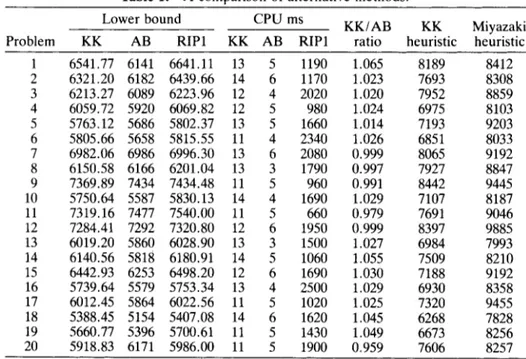
In Table 1 we compare the tightness of our bounds with those of Ahmadi and Bagchi [l], which are the best currently available. Ahmadi and Bagchi [ l ] bounds (AB bounds) are an improved version of Bansal's [3] m machine based bounds. The overall complexity of A B bounds is O(mn log n ) . The worst-case complexity of our bounds, on the other hand, is O(k(n3

+

IT*[)), where k is the number of iterations in the subgradient method. Note that at each iteration the multiplier vector A can be updated in O(lT*l) time.

We have generated 20 12-job six-machine problems using integer processing times drawn from a uniform (1-100) distribution. For each problem we have generated eight machine based path vectors, i.e., 1T*l = 8. A machine based path for position i in the schedule u is given as (t(i, j) = k , j = 1, . . . , i -

l ) , where 1 5 k 5 m. We have run the subgradient optimization method for

four iterations, i.e.

,

we have solved four consecutive linear assignment problems. The linear assignment solution procedure used is that of Tomizawa

[

171 and we

Table 1. A comparison of alternative methods.

cpu

ms KK/AB KK Miyazaki

Problem KK AB RIPl KK A B RIPl ratio heuristic heuristic Lower bound 1 2 3 4 5 6 7 8 9 10 11 12 13 14 15 16 17 18 19 20 6541.77 6321.20 6213.27 6059.72 5763.12 5805.66 6982.06 6150.58 7369.89 5750.64 7319.16 7284.41 60 19.20 6140.56 6442.93 5739.64 6012.45 5388.45 5660.77 591 8.83 6141 6182 6089 5920 5686 5658 6986 6166 7434 5587 7477 7292 5860 5818 6253 5579 5864 5154 5396 6171 6641.11 6439.66 6223.96 6069.82 5802.37 5815.55 6996.30 6201.04 7434.48 5830.13 7540.00 7320.80 6028.90 6180.91 6498.20 5753.34 6022.56 5407.08 5700.6 1 5986.00 13 5 1190 1.065 14 6 1170 1.023 12 4 2020 1.020 12 5 980 1.024 13 5 1660 1.014 11 4 2340 1.026 13 6 2080 0.999 13 3 1790 0.997 11 5 960 0.991 14 4 1690 1.029 11 5 660 0.979 12 6 1950 0.999 13 3 1500 1.027 14 5 1060 1.055 12 6 1690 1.030 13 4 2500 1.029 11 5 1020 1.025 14 6 1620 1.045 11 5 1430 1.049 11 5 1900 0.959 8189 7693 7952 6975 7193 685 1 8065 7927 8442 7107 7691 8397 6984 7509 7188 6930 7320 6268 6673 7606 ~ 8412 8308 8859 8103 9203 8033 9192 8847 9445 8187 9046 9885 7993 8210 9192 8358 9455 7828 8256 8257

have used the code developed by Burkard and Derigs [4]. The initial A vector is taken as

and

p'

is set equal to 25.0/(t

+

1)*, t 2 0.

In Table 1, Column 1 tabulates the lower bounds generated by the subgradient method. A B bounds are presented in Column 2. Optimal solution to the linear programming relaxation of the (RIP1) problem is documented in Column 3. A comparison of Columns 1 and 3 demonstrates the rapid convergence of the subgradient method. Columns 4-6 tabulate the CPU times for these three dif- ferent approaches (i.e., our subgradient procedure, the A B bounding scheme, and the solution of the linear programming relaxation of (RIP1) using the DDLPRS subroutine of IMSL). In Column 7 we present the ratio of our bounds to AB bounds. The average improvement is 1.9%, and in 14 problems our bounds have been strictly greater than the AB bounds. In Column 8 we report on the best upper bound obtained after four iterations of the subgradient ap- proach. Note that at each iteration of the subgradient procedure we solve a linear assignment problem, and the solution of this problem is a feasible schedule for the n / m / P / C C, problem. We refer to the best schedule generated in four iterations of the subgradient approach as our heuristic solution (i.e., the KK heuristic) to the problem. Finally in Column 9, the performance of the heuristic developed by Miyazaki et al. [ l l ] is tabulated. (The average performance of the KK heuristic is 16.5% better than that of Miyazaki heuristic.)

The overall performance of our approach is very promising. We can generate very good upper bounds (i.e., feasible schedules to the problem) while improving the currently available lower-bounding scheme. Note that A B bounds are ob- tained by generating a preemptive schedule for an n-job one-machine problem with ready times and sum of completion times criterion (i.e., n / l / r , 2 O/C C ,

problem). Therefore, the schedule that provides the lower bound in the AB method is not necessarily a feasible schedule for the original n/mlP/C C, prob- lem.

However, the two approaches, i.e., our subgradient method and A B bounds, differ in terms of their worst-case computational complexities, and we will ad- dress the tradeoff between goodness of a lower bound and its computational complexity in Section 6, where we compare the performances of these two approaches when they are embedded in an implicit enumeration scheme.

5. A NEW BRANCH-AND-BOUND APPROACH TO THE

nlmlPIZ Ci PROBLEM

Most research on optimal algorithm development for non-preemptive per- mutation flow shops has focused on enumerative methods. In this section we present a new branch-and-bound approach to the n / m / PIC C j problem.

Most of the enumerative approaches for permutation flow shop problems use as a branching scheme the assignment of jobs to the Ith position in the schedule

856 Naval Research Logistics, Vol. 40 (1993)

at the fth level of the search tree. Thus, at a node at that level a partial schedule (a(1). a(2),

. . . ,

~ ( 1 ) ) has been formed. The bounding scheme generates lower bounds on the value of all possible completions of the partial schedule. As will become clear from the description below, our branching-and-bounding schemes are distinctively different than those previously discussed in the literature.

BRANCHING SCHEME: Let S be a set of schedules and uo be a schedule in S. Then the set S\{ao} can be divided into at most n - 1 nonempty, mutually exclusive, and collectively exhaustive subsets as follows.

SI

= { a

E

S and a(1) # a-o(l)},

S 2 = { a

E

_{S and a(1) = q)(l), 4 2 ) # a0(2)},}

S3 = {a-E S and a(1) = q,(l), 4 2 ) = a0(2), u(3) # q , ( 3 ) } ,

and

S,,-l = { a € S and a(1) = vI(l),

. . .

, a(n - 1) # ao(n - 1)). The above sets S , , Sz,

. . .

,

S,-l

satisfy the above-mentioned properties, i.e.,

BOUNDING SCHEME: Let S be a set of schedules. Using the results of Section 4 we can conclude that the solutions to the (LRAP(A)) problem, subject to the constraint that the resulting schedule is in S, provide lower bounds for this particular set S. Due to the special structure of our branching scheme, the above-mentioned constraints can be easily incorporated into the objective func- tion, so that the resulting assignments (or schedules) are in S. For example, if a(1) # ~ ~ ( 1 ) in S, then we set u ; , , ( ~ ) . ~ = B, 7 E T* during the solution of ( L R A P ( A ) ) , where B is arbitrarily large.

At each node, we choose (T*I path vectors for lower-bound generation. In the current version of the algorithm, the path vector set T* contains different combinations of machine based paths for different positions in the schedule. For example, for location

i

in the schedule, the following set of integers is a machine based path: (t(i, j ) = k , k , j = 1, .

.

. ,

i

- 1) where 1 9 k 9 rn. However, as we move down in the search tree, the number of fixed jobs increases, and partial schedules of significant size are formed. Then, the set T* is formed in a way that the selected paths attain the maximum possible value on these partial sched- ules.

The performance of our algorithm is very much affected by the selection of the initial multiplier vector A in the subgradient optimization method. Due to the above-mentioned selection of T * , the path vector sets of a node and its children nodes are very similar, and in most cases the multiplier vector obtained

in the last iteration of the subgradient method is a very good initial multiplier vector for the children nodes of this particular node.

For each new subset of schedules generated, i.e., each node in our search tree, we use the same approach in developing lower and upper bounds. The iterations of the subgradient method provide us with lower bounds and feasible schedules. The sum of completion times of these schedules give us new upper bounds.

FATHOMING CRITERION: If the current upper bound is less than or equal to the lower bound on that subset of schedules.

NODE T O EXAMINE NEXT CRITERION: In the current version of our algorithm we examine next the subset of schedules that has the smallest lower bound.

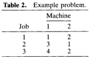
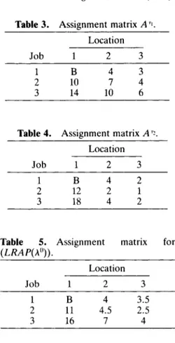
EXAMPLE: We will illustrate the basic ideas of the algorithm using the three-job and two-machine problem given in Table 2. Let S be the set of all schedules such that a(1) # 1, i.e., S = ((2, 1, 3 ) , (2, 3 , l ) , ( 3 , 1, 2), ( 3 , 2, l)}. Let IT:'[ = 2, and let rl and r2 be given as follows:

The assignment matrices A'' and A"- for S are given in Tables 3 and 4. Let A" =

(4, 4).

Then the assignment matrix for (LRAP(A2)) is as given in Table 5 . The solution of assignment problem is (T = (2, 1, 3 ) and fAp(AO) is equal to 19.

Now, the subgradient is given by p = (20 - 19, 18 - 19) = (1, -1). We can

also find an upper bound by computing the sum of completion times of schedule

(T, which is 20. Let

Po

= 2.5; then the new multiplier vector, before the nor-

malization, is given by

2.5(1)(20 ,>- " I

{

1 2 S - 1 ) ( 2 0 - 19) 2

max 0, -

+

2 2

or

1

= (1.75, 0), and therefore A' = (1, 0). In the next iteration we solve the linear assignment problem on the matrix A'', and the optimal solution is (T =

(2, 1, 3 ) and fAP(A1) = 20, which is equal to the upper bound. Therefore, for the set of schedules S , (T = (2, 1, 3 ) is an optimal schedule.

Table 2. Example problem.

Machine

Job 1 2

1 1 2

2 3 1

858 Naval Research Logistics, Vol. 40 (1993)

Table 3. Assignment matrix A'l.

Location

Job 1 2 3

1 B 4 3

2 10 7 4

3 14 10 6

Table 4. Assignment matrix AT?.

Location

Job 1 2 3

1 B 4 2

2 12 2 1

3 18 4 2

Table 5. Assignment matrix for

( LRA P( A")). Location Job 1 2 3 1 B 4 3.5 2 11 4.5 2.5 3 16 7 4

6. COMPUTATIONAL PERFORMANCE OF THE BRANCH-AND-

BOUND PROCEDURE

We have tested the performance of our algorithm using randomly generated problems. The method of problem generation follows that given in Lageweg, Lenstra, and Rinnooy Ken [9]; i.e., four different problem classes are consid- ered: random problems, problems with correlation between the processing times of each job, problems for which the processing times of each job have a positive trend, and finally problems with both correlation and positive trend. In Table 6 we present the distributions of these classes, where c(i) is the correlation coefficient of job i , i = 1,

. . . ,

n , with a uniform [0-41 distribution, and j is

the machine index.

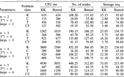
In Tables 7 and 8 we present the results comparing the performance of our branch-and-bound procedure to the one developed by Bansal [3], with the im- proved lower bounds of Ahmadi and Bagchi [l], for n = 8 and n = 10, re- spectively. Bansal's algorithm is a general approach which works with partial assignments, as described in the beginning of this section. Since A B bounds dominate the bounds developed by Bansal, we have used the improved bounds in the implementation of this approach. Both methods have been coded in FORTRAN, on a multiuser IBM 3081-D system.

In Tables 7 and 8 Column 1 documents the parameters of a specific set of problems, where m is the number of machines,

I

T*l is the number of path vectors

Table 6. Problem classes.

Problem class Distribution Parameters

Random (R) Uniform 1,100

Correlation (C) Uniform 20c(i)

+

1, 20c(i)

+

20 Trend (T) Correlation/trend (CT) Uniform Uniform 12.5(j - 1)

+

1, 12.5(j - 1)

+

100 2.5(j - 1)

+

2 0 4 4

+

1, 2.5(j - 1)

+

20c(i)

+

20

Table 7. Comparison of branch-and-bound methods for n = 8.

CPU ms No. of nodes Storage req.

Problem

Parameters class KK Bansal KK Bansal KK Bansal

R 619 624 108.20 131.65 15.15 95.65 C 115 286 18.05 53.40 2.80 34.30 m = 2 T 456 516 78.45 102.80 11.40 74.80 IT*[ = 3 CT 127 302 19.35 52.50 3.40 40.55 Steps = 2 m = 3 /T*l = 4 Steps = 3 m = 4 IT*\ = 5 Steps = 3 m = 5 IT*[ = 6 Steps = 4 R C T CT R C T CT R C T CT 1262 268 92 1 268 3860 289 920 609 4930 447 1604 1055 1019 506 677 452 2584 500 608 745 305 1 682 1104 1074 190.15 43.70 135.80 41.15 452.10 34.20 108.25 76.15 448.25 40.65 151.25 99.95 186.25 85.25 127.45 76.05 366.45 61.30 79.55 100.75 312.85 64.55 114.15 108.65 23.05 5.75 16.20 5.70 58.25 5.50 12.50 11.10 53.05 6.70 19.75 13.80

Table 8. Comparison of branch-and-bound methods for n = 10.

134.75 65.60 85.80 58.60 236.65 43.60 57.55 68.20 215.40 44.35 80.00 76.20

CPU ms No. of nodes Storage req.

Problem

Parameters class KK Bansal KK Bansal KK Bansal

R 6,119 7,381 714.84 C 461 672 52.75 T 4,199 5,337 491.25 CT 562 808 76.15 R 10,045 8,094 1,095.95 C 673 1,140 69.95 T 6,183 5,107 699.10 CT 2,575 3,354 302.35 R 28,602 25,396 2,233.75 C 2,064 3,281 211.05 T 5,705 4,510 562.80 2,636 3,056 231.05 m = 2 IT*[ = 3 Steps = 3 m = 3 IT*l = 4 Steps = 3 m = 4 IT*/ = 5 Steps = 3 CT R 44,903 32,797 3,394.10 C 2,281 3,298 176.55 T 6,163 4,600 485.00 CT 5.859 7.514 472.90 m = 5 IT*l = 6 Steps = 4 1,009.70 129.75 675.70 169.85 883.50 141.80 590.80 412.15 1,783.65 290.40 406.45 270.40 2,515.55 241.30 312.80 544.30 75.25 6.45 61.50 9.45 102.45 9.65 63.65 30.10 197.75 25.40 56.70 24.45 304.85 22.00 50.20 59.65 785.80 106.25 524.50 128.30 681.10 112.70 473.25 325.45 1,416.25 28.20 324.15 210.70 1,977.00 186.05 251.55 418.65

860 Naval Research Logistics, Vol. 40 (1993)

used in our lower-bound generation scheme and “Steps” is the number of it- erations in the subgradient method. Column 2 of Tables 7 and 8 denotes the problem class. For each class we have generated 20 problems; hence each entry in Tables 7 and 8 represents the average of 20 problems. In Columns 3 and 4 of Tables 7 and 8, we compare the computational effort required by our method (KK) and by Bansal’s procedure, respectively. In Columns 5 and 6 we present the average number of nodes generated by the two different approaches. In Columns 7 and 8, we report the average maximum number of nodes stored by our method, and by Bansal’s method, respectively. Note that the maximum number of nodes stored denotes the maximum number of active nodes (i.e., nodes that have been generated but not eliminated) at any time point during the actual run of the branch-and-bound procedure. This could be an important factor for large-size problems, especially if the storage constraints are more pressing than the CPU time constraint.

In two-machine eight-job and two-machine ten-job problems our approach dominates Bansal’s method, in terms of both CPU times and the number of nodes, in all of the four problem classes. For rn = 3, 4, and 5 , our method dominates Bansal’s approach in problems with correlation (C), and with cor- relation and trend (CT). In random problems (R) and problems with trend (T), Bansal’s method dominates our approach. Apparently for these problems the subgradient method cannot generate a good approximation of

f F P ,

within the allowed number of iterations. Increasing the number of iterations in the subgra- dient method has resulted in larger CPU times, although the number of nodes generated by our approach dominated that of Bansal’s method for some prob- lems in classes (R) and (T). In all problems our approach has dominated Bansal’s method in terms of storage requirement. The dominance of our method in this category also indicates that our approach generates very good upper bounds early in the search tree so that the number of active nodes is kept at a minimum level.

In order to illustrate the relative importance of this property, we have used our optimal method as a heuristic for large size problems. In Table 9, we doc-

Table 9.

Stopping Problem No. of Storage UB - L B

Heuristic run of the optimal algorithm.

Parameters criterion class c p u ms nodes req. L B

n = 20 m = 5 IT”1 = 6 Steps = 5 n = 25 m = 5 IT*/ = 6 Steps = 5 n = 30 m = 5 IT*l = 6 Steps = 5 CPU 5,000 or U B - L B 5 0.02 L B CPU 2 7,500 or UB - L B 5 0.02 L B CPU 2 12,500 or UB - L B 5 0.02 L B R C T CT R C T CT R C T CT 5,000 1,946 5,000 4,615 7,500 3,093 6,849 7,500 12,500 7,476 11,657 12,500 508.45 145.90 508.89 446.95 512.50 138.55 488.35 510.05 513.10 215.45 514.20 487.70 202.20 81.55 105.45 244.00 214.65 89.45 110.10 292.05 243.65 136.35 119.90 283.50 0.1716 0.0192 0.0601 0.0312 0.1797 0.0170 0.0599 0.0378 0.1888 0.0188 0.0801 0.0363

ument the performance of the heuristic run of our optimal method. In Table 9, Column 1 tabulates the parameters of a specific set of problems. Column 2 documents the stopping criterion used in the heuristic run of our optimal al- gorithm. For example, in 20-job five-machine problems, we have terminated the optimal algorithm when the total CPU time exceeded 5000 ms or when we found an upper bound which was within 2% of the lower bound. Column 3 documents the different problem classes. For each class we have generated 20 problems, and each entry represents the average of 20 problems. The average CPU time, number of nodes generated, and maximum number of nodes stored for each problem class are presented in Columns 4-6, respectively. In Column 7, we report the average performance of the heuristic run of the our optimal approach. Except for random problems, the heuristic has performed exception- ally well.

We have also used Bansal’s approach for the same problems; however, the only complete schedules generated by the Bansal’s method with the A B bounds have been the schedules generated when developing the lower bounds on the first machine, and the heuristic schedules developed by our approach dominated all of these schedules.

7. CONCLUSION

In this article we have developed a new modeling framework for the per- mutation flow shop scheduling problem for the minimization of the sum of completion times. The modeling framework is based on a game-theoretic inter- pretation of the problem. A Lagrangian relaxation approach on the resulting integer programming formulation is used to develop lower bounds for the prob- lem. Those bounds are implemented in an efficient branch-and-bound algorithm. The methodology developed in this article is quite flexible and it can handle, with minor modifications, a more general class of problems for the sum-of- completion-times criterion in permutation flow shops: the class of scheduling problems with finite buffer capacities. We have already undertaken research in this direction and we will report our research progress on these problems in a subsequent article.

REFERENCES

[ l ] Ahmadi, R.H., and Bagchi, U., “Improved Lower Bounds for Minimizing the Sum of Completion Times of n Jobs over m Machines in a Flow Shop,” European Journal of Operational Research, 44, 331-336 (1990).

[2] Baker, K.R., “A Comparative Study of Flow Shop Algorithms,” Operations Re- search, 23(2), 62-73 (1975).

[3] Bansal, S.P., “Minimizing the Sum of Completion Times of n Jobs over m Machines in a Flow Shop-a Branch-and-Bound Algorithm,” AIIE, 9 , 306-31 1 (1977).

[4] Burkard, R.E., and Derigs, U., Assignment and Matching Problems: Solution Meth- ods with FORTRAN Programs, Springer-Verlag, Berlin, 1980.

[5] Goffin, J.L., “On Convergence Rates of Subgradient Optimization Methods,” Math- ematical Programming, 13, 329-347 (1977).

[6] Gonzalez, T., and Sahni, S . , “Flow Shop and Job Shop Schedules: Complexity and Approximation,” Operations Research, 26( l ), 36-52 (1978).

862 Naval Research Logistics, Vol. 40 (1993)

[7] Ignall, E., and Schrage, L.E., “Application of the Branch-and-Bound Technique to Some Flow Shop Problems,” Operations Research, 13, 400-412 (1965). [8] Kohler, W.H., and Steiglitz, K., “Exact, Approgmate, and Guaranteed Accuracy

Algorithms for the Flow Shop Problem nlmlFIF,” Journal of the Association for

Computing Machinery, 22, 106-114 (1975).

[9] Lageweg, B.J., Lenstra, J.K., and Rinnooy Kan, A.H.G., “A General Bounding Scheme for the Permutation Flowshop,” Operations Research, 26, 53-67 (1978). [lo] Lawler, E.L., Combinatorial Optimization: Networks and Matroids, Rinehart and

Winston, 1976.

[ l l ] Miyazaki, S . , Nishiyama, N., and Hashimoto, F., “An Adjacent Pairwise Inter- change Approach to the Mean Flow Time Scheduling Problem,” Journal of the

Operations Research Society of Japan, 21(2), 287-299 (1978).

[12] Monma, C.L., and Rinnooy Kan, A.H.G., “A Concise Survey of Efficiently Solvable Special Cases of the Permutation Flowshop Problem,” R A I R O , 17, 105-119 (1983). [13] Nemhauser, G.L., and Wolsey, L.A., Integer and Combinatorial Optimization, John

Wiley and Sons, New York, 1988.

[14] Panwalkar, S.S., and Khan, A.W., “An Ordered Flow Shop Sequencing Problem with Mean Completion Time Criterion,” International Journal of Production Re-

search, 14(5), 631-635 ‘(1976).

[ 151 Szwarc, W., “Permutation Flowshop Theory Revisited,” Naval Research Logistics

Quarterly, 26, 557-570 (1978).

1161 Szwarc, W., “The Flow Shop Problem with Mean Completion Time Criterion,” IIE

Transactions, 15(2), 172-176 (1983).

[17] Tomizawa, N., “On Some Techniques Useful for Solution of Transportation Net- work Problems,” Networks, 2, 179-194 (1972).

[18] von Neumann, J., and Morgenstern, O., Theory of Games and Economic Behavior, Princeton University Press, Princeton, NJ, 1947.

Manuscript received April 29, 1991

Revised manuscript received December 31, 1992 Accepted April 27, 1993