Please cite this article as: H. B. Jond, J. Platoš, Z. Sadreddini, Autonomous Vehicle Convoy Formation Control with Size/Shape Switching for Automated Highways, International Journal of Engineering (IJE), IJE TRANSACTIONS B: Applications Vol. 33, No. 11, (November 2020) 2174-2180
International Journal of Engineering
J o u r n a l H o m e p a g e : w w w . i j e . i rAutonomous Vehicle Convoy Formation Control with Size/Shape Switching for
Automated Highways
H. B. Jond*a, J. Platoša, Z. Sadreddinib
a Department of Computer Science, VSB – Technical University of Ostrava, Ostrava, Czech Republic b Department of Computer Engineering, Istanbul Arel University, Istanbul, Turkey
P A P E R I N F O Paper history: Received 15 April 2020
Received in revised form 03 September 2020 Accepted 03 September 2020
Keywords:
Automated Highway Autonomous Vehicle Formation Control Receding Horizon Control Size/Shape Switching
A B S T R A C T
Today’s semi-autonomous vehicles are gradually moving towards full autonomy. This transition requires developing effective control algorithms for handing complex autonomous tasks. Driving as a group of vehicles, referred to as a convoy, on automated highways is a highly important and challenging task that autonomous driving systems must deal with. This paper considers the control problem of a vehicle convoy modeled with linear dynamics. The convoy formation requirement is presented in terms of a quadratic performance index to minimize. The convoy formation control is formulated as a receding horizon linear-quadratic (LQ) optimal control problem.The receding horizon control law is innovatively defined via the solution to the algebraic Riccati equation.The solution matrix and therefore the receding horizon control law are obtained in the closed-form.A control architecture consisting of four algorithms is proposed to handle formation size/shape switching.The closed-form control law is at the core of these algorithms. Simulation results are provided to justify the models, solutions, and proposed algorithms.
doi: 10.5829/ije.2020.33.11b.07
1. INTRODUCTION1
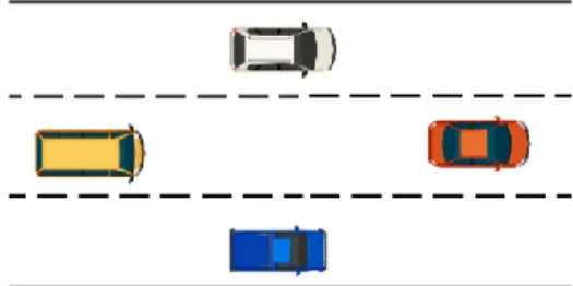
Soon, public roads will host the massive deployment of autonomous vehicles. An autonomous convoy is a group of networked autonomous vehicles maintaining a formation (Figure 1). The formation control is defined as designing control inputs for the vehicles so that they form and maintain a pre-defined geometric shape. The line (or linear) formation, so-called platooning, concerns only longitudinal coordinated control of networked autonomous vehicles [1]. Convoy formation control requires both longitudinal and lateral coordination of vehicles [2]. Convoy control algorithms are essential for vehicle maneuvers such as lane change and overtaking on automated highways. Intelligent Traffic Management Systems [3] can also use these algorithms for city traffic.
Many algorithms from multi-agent systems are used in autonomous vehicle convoy formation control. Classical approaches which include leader-follower [4], virtual-structure [5] and behavior-based [6, 7] comprise a
*Corresponding Author Institutional Email: [email protected] (H. B. Jond)
significant amount of research effort in multi-agent systems formation control.
While the leader-follower approach is a popular design for the formation control, there are limitations. The loss of the leader or the leader being perturbed by some disturbances causes the entire group formation to fail [8]. On the contrary, the formation control can be leaderless, where all agents have the same role within the team.
In this study, we intend to derive an optimality-based formation control strategy for a leaderless autonomous
convoy. The optimality-based approach has received attention in robotic car literature (see, e.g., [9, 10]). Particularly the LQ modeling of formation control is highly interesting due to the analytic tractability of LQ problems. In this approach, the formation objective, which is to drive multiple agents to achieve a prescribed constraint on their states, is implemented by using a quadratic performance index through the use of graph theory [11]. The multi-agent system dynamics is modeled as a controllable linear system.
Depending on the available information structure, open-loop [12], state-feedback [13] and receding horizon [14] control structures can be investigated for formation control. The receding horizon or model predictive controller uses the open-loop control signals to implement an online algorithm that predicts the system’s output based on current states and system models. It has become the most popular feedback strategy in industrial applications.
In the operation field, when obstacles or boundaries are detected along the formation's path, the formation is able to squeeze through obstacles by switching to suited patterns that are chosen among a collection of formations. In some other cases, a safe formation control strategy scales the formation shape (by a size switching strategy). By adjusting the scale, the formation can grow and shrink as necessary to accommodate and avoid obstacles in it’s surrounding area. An illustrative example is given in [15], where a group of agents is to traverse a narrow passage while maintaining a desired triangular shape.
In this paper, the convoy formation control is addressed as a receding horizon LQ optimal control problem. Under this framework, the matrix Riccati equation must be solved. Obtaining a solution to this equation is not generally straightforward. This type of matrix equation has been discussed in detail in [16]. Innovatively, the receding horizon control law is constructed via the algebraic Riccati equation, which leads to obtaining the control law in the closed-form. Besides, a control scheme is developed to deal with the formation size/shape switching under the receding horizon LQ framework. This scheme consists of four control modes in which each control mode is run under an algorithm constructed via the closed-form control law.
The remainder of this paper is organized as follows. The system models and LQ optimal control formulation of the formation control problem are introduced in Section 2. The receding horizon control design is presented in Section 3. The control scheme and corresponding algorithms for formation size/shape switching are developed in Section 4. The simulation results are shown in Section 5. The conclusion is given in Section 6.
2. CONVOY FORMATION STATEMENT
Vehicle dynamics is highly nonlinear. Hierarchical control architectures at their top-level consider a simplified dynamics model of the system and shift the nonlinearity to their lower levels. An appropriate simple dynamical model for a vehicle is the double integrator model. It simplifies vehicle dynamics as a point mass governed by Newton’s laws [17].
Consider a convoy of 𝑚 networked vehicles, each of which is described by a double integrator dynamics. Let 𝒒𝑖, 𝒗𝑖, 𝒖𝑖∈ ℝ2 be the coordinates, velocity and control input vectors for vehicle 𝑖 (𝑖 = 1, … , 𝑚), respectively. Define 𝒛 = [𝒒1𝑇, … , 𝒒𝑚𝑇, 1, 𝒗1𝑇, … , 𝒗𝑚𝑇]𝑇 and 𝒖 = [𝒖1𝑇, … , 𝒖𝑚𝑇]𝑇. Vectors 𝒛 ∈ ℝ4𝑚+1 and 𝒖 ∈ ℝ2𝑚 are system state and control input vectors, respectively. The system dynamics can be expressed as
𝒛̇ = 𝑨𝒛 + 𝑩𝒖 (1)
where 𝑨 = [𝟎 𝑰𝟐𝒎
𝟎 𝟎 ], 𝑩 = [𝟎𝟐𝒎, 𝟎𝟐𝒎×𝟏, 𝑰𝟐𝒎]
𝑻, and 𝑰 is the identity matrix of appropriate dimension.
Networked systems such as a convoy of vehicles exchange information via a communication network. The information flow over the communication network can be modeled with graph theory. A directed graph 𝒢 = (𝒱, ℰ) consists of a set of vertices 𝒱 = {1,2, … , 𝑚} and a set of edges ℰ ⊆ {(𝑖, 𝑗): 𝑖, 𝑗 ∈ 𝒱} containing ordered pairs of distinct vertices. For the formation control, the set of vertices 𝒱 corresponds to the vehicles and then the set of edges ℰ represents the interconnections. Each edge (𝑖, 𝑗) ∈ ℰ is assigned with a weight 𝜇𝑖𝑗> 0.
Assumption 1. Formation graph 𝒢 is connected, i.e., for every pair of vertices i j ∈ 𝒱, from i to j for all j = 1 , , , m, j ≠ i, there exists a path of (undirected) edges from ℰ.
The graph Laplacian 𝑳 ∈ ℝ𝑚 is defined as
𝑳 = 𝑫𝑾𝑫𝑇 (2)
where 𝑫 ∈ ℝ𝑚×|ℰ| is the incidence matrix and 𝑾 = 𝑑𝑖𝑎𝑔(𝜇𝑖𝑗) ∈ ℝ|ℰ| is a diagonal weight matrix. 𝑫's 𝑢𝑣th element is 1 if the node 𝑢 is the head of the edge 𝑣, -1 if the node 𝑢 is the tail, and 0, otherwise.
The Kronecker product ⨂ can be used to extend the dimension. The 2-dimensional graph Laplacian 𝓛 ∈ ℝ2𝑚 is defined as
𝓛 = 𝑳⨂𝑰2 (3)
Based on the properties of the Kronecker product, 𝓛 can be rearranged as 𝓛 = 𝑫𝑾𝑫𝑇⊗ 𝑰 2= (𝑫 ⊗ 𝑰2)(𝑾 ⊗ 𝑰2)(𝑫 ⊗ 𝑰2)𝑇= 𝓓𝓦𝓓𝑇 (4) where 𝓓 = 𝑫 ⊗ 𝑰2 and 𝓦 = 𝑾 ⊗ 𝑰2.
The graph Laplacian is symmetric, positive semidefinite and holds the sum-of-squares property [18]:
𝒛𝑻𝓛𝒛 = ∑ 𝜇
𝑖𝑗‖𝒒𝑖− 𝒒𝑗‖ 𝟐
(𝑖,𝑗)∈ℰ (5)
where ‖. ‖ is the Euclidean norm in ℝ2.
The formation requirement according to the information graph can be expressed as
∑ 𝜇𝑖𝑗(‖𝒒𝑖− 𝒒𝑗− 𝒅𝑖𝑗‖ 2 + ‖𝒗𝑖− 𝒗𝑗‖ 2 ) (𝑖,𝑗)𝜖ℰ → 0 (6)
where 𝒅𝑖𝑗 ∈ ℝ𝑛 is the desired distance vector between two neighbor vehicles 𝑖 and 𝑗. Using the property of sum-of-squares, (6) can be transformed into the following matrix form ∑ 𝜔𝑖𝑗(‖𝒒𝑖− 𝒒𝑗‖ 2 − 2(𝒒𝑖− 𝒒𝑗) 𝑇 𝒅𝑖𝑗+ (𝑖,𝑗)𝜖ℰ ‖𝒅𝑖𝑗‖ 2 + ‖𝒗𝑖− 𝒗𝑗‖ 2 ) = 𝒒𝑇𝓛𝒒 − 2𝒒𝑇𝓓𝓦𝒅 + 𝒅𝑇𝓦𝒅 + 𝒗𝑇𝓛𝒗 = 𝒛𝑇𝑸𝒛 (7) where 𝑸 = [ 𝓛 −𝓓𝓦𝒅 𝟎 −(𝓓𝓦𝒅)𝑻 𝒅𝑻𝓦𝒅 𝟎 𝟎 𝟎 𝓛 ], 𝒅 = 𝑐𝑜𝑙(𝒅𝑖𝑗) and 𝑐𝑜𝑙(. ) stands for "column vector". As 𝒛𝑇𝑸𝒛 ≥ 0, matrix 𝑸 is positive semidefinite.
A performance index for the convoy formation control is defined as 𝐽 = 𝒛(𝑡𝑓) 𝑇 𝑸𝑓𝒛(𝑡𝑓) + ∫ (𝒛𝑇𝑸𝒛 + 𝒖𝑇𝑹𝒖)𝑑𝑡 𝑡𝑓 0 (8) where 𝑸𝒇= [ 𝓛𝒇 −𝓓𝓦𝒇𝒅 𝟎 −(𝓓𝓦𝒇𝒅) 𝑻 𝒅𝑻𝓦 𝒇𝒅 𝟎 𝟎 𝟎 𝓛𝒇 ], 𝓛𝑓= 𝓓𝓦𝑓𝓓𝑇, 𝓦𝑓= 𝑾𝑓⊗ 𝑰𝑛, 𝑾𝑓 = 𝑑𝑖𝑎𝑔(𝜔𝑖𝑗) ∈ ℝ|ℰ|, 𝜔𝑖𝑗 > 0, 𝑡𝑓 is the fixed finite horizon length and 𝑹 ∈ ℝ2𝑚 is diagonal positive definite (𝑹 > 𝟎). Matrices 𝑾 and 𝑹 represent the penalties on the formation-velocity errors and control effort during the entire formation control process, respectively. Matrix 𝑾𝑓 represents the penalty on the terminal formation-velocity errors.
The convoy formation control objective is to design the control input vector 𝒖 to minimize the performance index 𝐽 for the underlying system dynamics (1). The formation control problem under the framework of LQ optimal control formulation converts to the symmetric Riccati differential equation problem, which is stated in the following theorem. The proof can be found in [19].
Theorem 1. For the formation control defined as the LQ
optimal control problem (1) and (8), the open-loop solution is given by
𝒖 = −𝑹−1𝑩𝑇𝑷𝒛 (9)
where 𝑷 is the solution to the Riccati differential equation;
𝑷̇ + 𝑷𝑨 + 𝑨𝑇𝑷 − 𝑷𝑺𝑷 + 𝑸 = 𝟎, 𝑷(𝑡
𝑓) = 𝑸𝑓 (10) and 𝑆 = 𝐵𝑅−1𝐵𝑇.
Matrix 𝑷 is symmetric positive semidefinite. In general, (10) must be solved numerically by using the terminal value and backward iteration.
3. RECEDING HORIZON CONTROL
Fixed horizon control problems suffer from the main drawback that unexpected changes in the system that may happen at a future time cannot be included in the model. This issue is addressed by the idea of receding horizon control [20]. Let 0 < 𝛿 < 𝑡𝑓 denote the sampling period. In the receding horizon control, the current control law 𝒖 is obtained by solving the open-loop optimal control problem (1) and (8) at each sampling instant 𝑡 for the interval [𝑡, 𝑡 + 𝑡𝑓]. Then, 𝒖 and the corresponding system trajectory 𝒛 is used until the next sampling time 𝑡 + 𝛿 arrives. In this method, at each time instant 𝑡 the current state vector 𝒛 is considered as the initial state. The open-loop control signal 𝒖 minimizes the following receding horizon performance index
𝐽̂ = 𝒛(𝑡 + 𝑡𝑓) 𝑇 𝑸𝑓𝒛(𝑡 + 𝑡𝑓) + ∫ (𝒛𝑇𝑸𝒛 + 𝑡+𝑡𝑓 𝑡 𝒖𝑇𝑹𝒖)𝑑𝜏 (11)
Following [14], the receding horizon control for the formation control problem is defined as
𝒖̅ = −𝑹−1𝑩𝑇𝑷(0)𝒛 (12)
The closed-loop system is
𝒛̇ = 𝑨𝑐𝑙(0)𝒛 (13)
where 𝑨𝑐𝑙(0) = 𝑨 − 𝑺𝑷(0) is the closed-loop system matrix.
As it is seen from (12) calculation of the signal 𝒖̅ needs the solution matrix 𝑷(0) of the Riccati differential Equation (10). In a particular case in which 𝑡𝑓→ ∞, 𝑷 approaches a finite constant 𝓟 where it satisfies the algebraic Riccati equation (ARE)
𝓟𝑨 + 𝑨𝑇𝓟 − 𝓟𝑺𝓟 + 𝑸 = 𝟎 (14)
In the system dynamics (1) if (𝑨, 𝑩) is stabilizable then 𝓟 is a stabilizing solution to (10). Moreover, 𝑷 approaches to 𝓟 as 𝑡 → −∞. Therefore, in this paper, we propose the idea that solution 𝓟 to the ARE (14) can be used in (12) instead of 𝑷(0). Consequently, the receding horizon control for the formation control problem in (1) and (11) is redefined as
𝒖̅ = −𝑹−1𝑩𝑇𝓟𝒛 (15)
In the next theorem, the closed-form solution of the algebraic Riccati Equation (14) is presented. Before, the following definition is introduced.
Definition 1. Let the real symmetric matrix 𝐌 be positive semidefinite. The square root of 𝐌 is denoted by 𝐌12 and
satisfies 𝐌 = 𝐌12𝐌 1
2. Any symmetric, positive semidefinite matrix has a unique symmetric, semidefinite square root [21].
Theorem 2. The unique symmetric solution to the
algebraic Riccati Equation (14) is in the following form: 𝓟 = [𝑴𝑹 −1𝑵 −𝑴𝑵−1𝓓𝓦𝒅 𝑵 ∗ ∗ ∗ 𝑵 −𝑹𝑵−1𝓓𝓦𝒅 𝑴 ] (16)
where 𝑴 = (2𝑵𝑹 + 𝑵2)12, 𝑵 = (𝓛𝑹)12 and ∗ are the elements/blocks to be not concerned.
Proof. By ignoring the (artificially made) middle row of
𝑨 we see that (𝑨, 𝑩) is stabilizable. As 𝑹 is positive definite, and 𝑸 is symmetric positive semidefinite, there exists a unique symmetric solution to (14).
Assume that 𝓟 has the following form:
𝓟 = [
𝓟11 𝓟12 𝓟13 𝓟12𝑇 𝒫22 𝓟23 𝓟13 𝓟23𝑇 𝓟33
] (17)
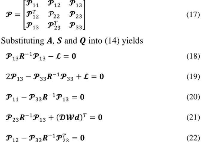
Substituting 𝑨, 𝑺 and 𝑸 into (14) yields
𝓟13𝑹−1𝓟13− 𝓛 = 𝟎 (18)
2𝓟13− 𝓟33𝑹−1𝓟33+ 𝓛 = 𝟎 (19)
𝓟11− 𝓟33𝑹−1𝓟13= 𝟎 (20)
𝓟23𝑹−1𝓟13+ (𝓓𝓦𝒅)𝑇= 𝟎 (21)
𝓟12− 𝓟33𝑹−1𝓟23𝑇 = 𝟎 (22)
By solving these equations using the matrix square root definition we obtain (16). Finally, from (15) it can be seen that the calculation of 𝒖̅ is not dependent on the middle row elements/blocks of 𝓟.
The closed-loop system matrix is redefined as 𝑨̅𝑐𝑙= 𝑨 − 𝑺𝓟. The system is asymptotically stable on the condition that all the eigenvalues of 𝑨̅𝑐𝑙 have negative real parts. As 𝑨̅𝑐𝑙 is a function of penalty matrices 𝑾 and 𝑹, the asymptotic stability can be achieved by selecting appropriate 𝑾 and 𝑹 matrices.
Together with satisfying the asymptotic stability condition, matrices 𝑾 and 𝑹 should reflect the real-world requirements such as vehicle's energy consumption management. For example, if the vehicles have a sufficient amount of fuel in their tank or if they are near a gas station, a large 𝑾 and a small 𝑹 can be selected to emphasize the formation-velocity errors rather than the control effort. On the contrary, a small 𝑾 and a large 𝑹 can be selected for situations in which the vehicles are on an energy-saving policy. The best trade-off between the system performance (e.g. convoy formation) and control effort (e.g. energy consumption) should be taken.
4. SIZE/SHAPE SWITCHING
The receding horizon based controller calculates controls that drive each vehicle to acquire the desired relative position with respect to it’s neighbor(s) in the graph topology. During the process of acquiring a desired formation shape, at every time instant, there could be a change in the environment/system that might require a new desired formation shape to be acquired. For example, due to newly detected obstacles or failed vehicle(s) in the group, the initial formation topology would be subject to change in size/shape.
To handle size/shape switching a control architecture is presented in Figure 2. Based on the signal received from an external observer or a decision-maker vehicle equipped with appropriate sensors, a control mode is selected at each time instant. The control loop terminates when the formation control expectations are fulfilled.
Initially, the vehicle convoy is supposed to acquire the desired formation under the receding horizon control scheme. The receding horizon approach to the formation control problem is implemented using Algorithm 1. Here, the control commands are generated by the closed-form law in (15).
Algorithm 1. Receding Horizon Control
At each time instant 𝑡:
1: Measure the current state vector 𝒛
2: Calculate 𝒖 and 𝒛 for [𝑡, 𝑡 + 𝑡𝑓]
3: Apply 𝒖 = 𝒖̅ for the period [𝑡, 𝑡 + 𝛿]
4: Update 𝑡 ← 𝑡 + 𝛿
5: Repeat the steps 1 to 4
Size switching is subject to change only at desired distances among neighboring vehicles. Within this control platform when a size switching signal is received the formation desired distances vector 𝒅 = 𝑐𝑜𝑙(𝒅𝑖𝑗) is multiplied by a scalar 𝛼 where 𝛼 is the formation shape scale factor. In this case, recalculation of the open-loop
control 𝒖 for [𝑡, 𝑡 + 𝑡𝑓] needs fewer computation resources. This is because the control signal can be rewritten as
𝒖 = −𝑹−1(𝑵𝒒−𝑹(𝑵−1)𝑇𝓓𝓦𝒅 + 𝑴𝒗) (23) and as it is seen only the middle term is subject to being multiplied by scalar 𝛼. The proposed size switching procedure is presented in Algorithm 2.
Algorithm 2. Size Switching
At each time instant 𝑡:
1: Measure the current state vector 𝒛(𝑡)
2: Update 𝒅 as 𝛼𝒅
3: Calculate 𝒖 and 𝒛 for [𝑡, 𝑡 + 𝑡𝑓]
4: Apply 𝒖 = 𝒖̅ for the period [𝑡, 𝑡 + 𝛿]
5: Update 𝑡 ← 𝑡 + 𝛿
6: Repeat the steps 1 to 5
In shape switching the vehicles might keep their neighbors but need to acquire different desired distances. In other words, formation graph 𝒢 does not change. In this case, similar to size switching only the middle term of the control signal is subject to the minor change of updating 𝒅. The proposed shape switching procedure is presented in Algorithm 3.
Algorithm 3. Shape Switching (𝒢 has not changed)
At each time instant 𝑡:
1: Measure the current state vector 𝒛(𝑡)
2: Update 𝒅
3: Calculate 𝒖 and 𝒛 for [𝑡, 𝑡 + 𝑡𝑓]
4: Apply 𝒖 = 𝒖̅ for the period [𝑡, 𝑡 + 𝛿]
5: Update 𝑡 ← 𝑡 + 𝛿
6: Repeat the steps 1 to 5
Shape switching might be subject to change on interconnections. Some vehicles might lose some of their immediate neighbors in the graph topology and some might acquire new neighbors (i.e., 𝒢 changes). Here, the 𝑫, 𝑾 and 𝒅 parameters of the control signal must be updated. The proposed shape switching procedure when 𝒢 changes, is presented in Algorithm 4.
Algorithm 4. Shape Switching ((𝒢 has changed)
At each time instant 𝑡:
1: Measure the current state vector 𝒛(𝑡)
2: Update 𝑫, 𝑾, 𝒅
3: Calculate 𝒖 and 𝒛 for [𝑡, 𝑡 + 𝑡𝑓]
4: Apply 𝒖 = 𝒖̅ for the period [𝑡, 𝑡 + 𝛿]
5: Update 𝑡 ← 𝑡 + 𝛿
6: Repeat the steps 1 to 5
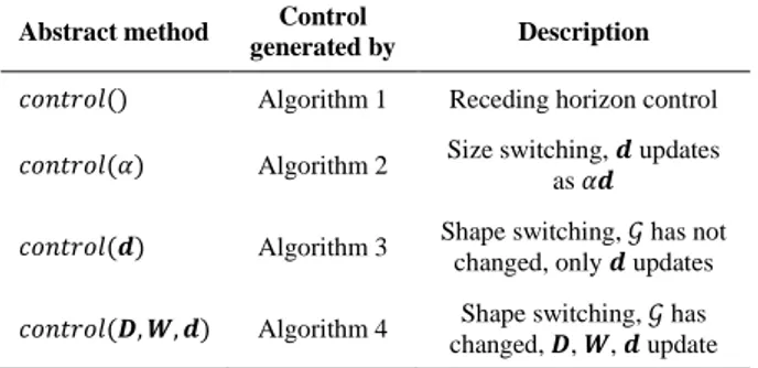
When designing the software interface of the control structure in Figure 2 (for example in Java), each different control mode can be addressed by using the abstract methods presented in Table 1.
TABLE 1. Abstract methods for different control procedures
Abstract method Control
generated by Description
𝑐𝑜𝑛𝑡𝑟𝑜𝑙() Algorithm 1 Receding horizon control 𝑐𝑜𝑛𝑡𝑟𝑜𝑙(𝛼) Algorithm 2 Size switching, 𝒅 updates as 𝛼𝒅 𝑐𝑜𝑛𝑡𝑟𝑜𝑙(𝒅) Algorithm 3 Shape switching, 𝒢 has not changed, only 𝒅 updates
𝑐𝑜𝑛𝑡𝑟𝑜𝑙(𝑫, 𝑾, 𝒅) Algorithm 4 Shape switching, 𝒢 has changed, 𝑫, 𝑾, 𝒅 update
5. SIMULATIONS
Simulations are carried out to analyze the proposed control architecture and algorithms. The experiments consist of five vehicles (𝑚 = 5). We consider a scenario in which at the time instants 𝑡 = 0𝑠 and 𝑡 = 7𝑠, the vehicles receive the signals 𝑐𝑜𝑛𝑡𝑟𝑜𝑙() and 𝑐𝑜𝑛𝑡𝑟𝑜𝑙(𝑫, 𝑾, 𝒅), respectively. The corresponding information graphs are given in Figure 3, and their incidence matrices are, respectively:
𝑫 = [ −1 −1 1 0 0 0 −1 0 0 0 0 1 0 0 1 0 0 −1 0 1 ] , 𝑫 = [ 0 −1 1 0 0 0 −1 0 0 0 −1 1 0 0 1 0 0 −1 0 1 ] .
The weight matrices 𝑾 and 𝑹 are selected as the identity matrices. The desired offset vectors of the formation shape among the vehicles at 𝑡 = 0𝑠 are: 𝒅12 = 𝒅23 = [−2, −4]𝑇 and 𝒅
14= 𝒅45= [2, −4]𝑇.These vectors mean that to form the desired shape; vehicle 1 and 2, as well as vehicle 2 and 3, have to achieve to relative distance -2 and -4 in the 𝑥 and 𝑦 position, respectively; vehicle 1 and 4, as well as vehicle 4 and 5, have to achieve to relative distance 2 and -4 in the 𝑥 and 𝑦 position, respectively. Moreover, all vehicles have to achieve zero relative velocities.
At time instant 𝑡 = 7𝑠, the communication link between vehicles 1 and 2 must break down and a new link between vehicles 2 and 4 must be built. The new desired offset vectors are: 𝒅24= [2,0]𝑇, 𝒅14= [2, −4]𝑇, 𝒅23 = 𝒅45= [0, −4]𝑇.
The initial positions of the vehicles are set to: 𝒒1= [1,0]𝑇, 𝒒
2= [4,0]𝑇, 𝒒3= [7,0]𝑇, 𝒒4= [−1,0]𝑇, 𝒒5= [−4,0]𝑇. The initial velocities are set to: 𝒒̇
1= [0,2]𝑇, 𝒒̇2= [0,3]𝑇, 𝒒̇
3= [0,1.5]𝑇, 𝒒̇4= [0,1]𝑇, 𝒒̇5= [0,2.5]𝑇.
The finite horizon length is selected as 𝑡𝑓 = 7𝑠 and the sampling time for simulation/control is 0,1𝑠. The total running time of the control is 14s. The vehicles’
trajectories under signals 𝑐𝑜𝑛𝑡𝑟𝑜𝑙() and
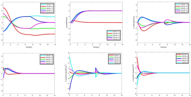
𝑐𝑜𝑛𝑡𝑟𝑜𝑙(𝑫, 𝑾, 𝒅) are shown in Figure 4. The vehicles are shown at 𝑡 = 0𝑠, 𝑡 = 5𝑠, and 𝑡 = 12𝑠. The results show that the desired formations among the vehicles are achieved under both signals at the end of their time interval. Time histories of the relative positions and velocities and also the control input of the individual vehicles are shown in Figure 5. It can be seen that all the formation control objectives are achieved.
Figure 4. Vehicles’ trajectories under 𝑐𝑜𝑛𝑡𝑟𝑜𝑙() followed
by 𝑐𝑜𝑛𝑡𝑟𝑜𝑙(𝑫, 𝑾, 𝒅) in red and blue, respectively
Figure 5. Time histories of the relative positions, velocities and control inputs under 𝑐𝑜𝑛𝑡𝑟𝑜𝑙() followed by 𝑐𝑜𝑛𝑡𝑟𝑜𝑙(𝑫, 𝑾, 𝒅)
6. CONCLUSION
In this paper, the convoy formation control problem was investigated under the receding horizon LQ optimal control framework. A closed-form solution was presented for the receding horizon LQ optimal formation control. The solution to the control law is a non-linear function of the graph Laplacian matrix and the formation desired distance vectors. A control architecture consisting of four control modes for formation size/shape switching problems was proposed. An algorithm based on the presented closed-form control law is developed for each control mode. The models, closed-form solution and proposed algorithms are approved by the simulations.
7. ACKNOWLEDGMENTS
This work was supported by the ESF in "Science without
borders" project, reg. nr.
CZ.02.2.69/0.0/0.0/16_027/0008463 within the Operational Programme Research, Development and Education.
8. REFERENCES
1. Chehardoli, H., and Homaienezhad, M. “Third-order Decentralized Safe Consensus Protocol for Inter-connected Heterogeneous Vehicular Platoons.” International Journal of
967–972. https://doi.org/10.5829/ije.2018.31.06c.14
2. Qian, X., De La Fortelle, A., and Moutarde, F. “A hierarchical Model Predictive Control framework for on-road formation control of autonomous vehicles.” In Proceedings IEEE Intelligent Vehicles Symposium, (Vol. 2016), 376–381. https://doi.org/10.1109/IVS.2016.7535413
3. Sumia, L., and Ranga, V. “Intelligent Traffic Management System for Prioritizing Emergency Vehicles in a Smart City.”
International Journal of Engineering - Transactions B:
Applications, Vol. 31, No. 2, (2018), 278–283.
https://doi.org/10.5829/ije.2018.31.02b.11
4. Liu, X., Ge, S. S., and Goh, C. H. “Vision-Based Leader-Follower Formation Control of Multiagents with Visibility Constraints.”
IEEE Transactions on Control Systems Technology, Vol. 27,
No. 3, (2019), 1326–1333.
https://doi.org/10.1109/TCST.2018.2790966
5. Rabelo, M. F. S., Brandao, A. S., and Sarcinelli-Filho, M. “Centralized control for an heterogeneous line formation using virtual structure approach.” In Proceedings - 15th Latin American Robotics Symposium, 6th Brazilian Robotics Symposium and 9th Workshop on Robotics in Education, LARS/SBR/WRE 2018, 141–146. https://doi.org/10.1109/LARS/SBR/WRE.2018.00033 6. Balch, T., and Arkin, R. C. “Behavior-based formation control for
multirobot teams.” IEEE Transactions on Robotics and
Automation, Vol. 14, No. 6, (1998), 926–939.
https://doi.org/10.1109/70.736776
7. Xu, D., Zhang, X., Zhu, Z., Chen, C., and Yang, P. “Behavior-based formation control of swarm robots.” Mathematical
Problems in Engineering, Vol. 2014, (2014), 1–13.
https://doi.org/10.1155/2014/205759
8. Ren, W., and Sorensen, N. “Distributed coordination architecture for multi-robot formation control.” Robotics and Autonomous
Systems, Vol. 56, No. 4, (2008), 324–333.
https://doi.org/10.1016/j.robot.2007.08.005
9. Wang, J., and Xin, M. “Integrated optimal formation control of multiple unmanned aerial vehicles.” IEEE Transactions on
Control Systems Technology, Vol. 21, No. 5, (2013), 1731–1744.
https://doi.org/10.1109/TCST.2012.2218815
10. Pourasad, Y. “Optimal Control of the Vehicle Path Following by Using Image Processing Approach.” International Journal of
Engineering - Transactions C: Aspects, Vol. 31, No. 9, (2018),
1559–1567. https://doi.org/10.5829/ije.2018.31.09c.12 11. Hossein Barghi Jond, Vasif V. Nabiyev, and Dalibor Lukáš.
“Linear Quadratic Differential Game Formulation for Leaderless Formation Control.” Journal of Industrial and Systems
Engineering, Vol. 11, , (2017), 47–58. Retrieved from
http://www.jise.ir/article_50882.html
12. Lin, W. “Distributed UAV formation control using differential game approach.” Aerospace Science and Technology, Vol. 35, No. 1, (2014), 54–62. https://doi.org/10.1016/j.ast.2014.02.004 13. Meng, Y., Chen, Q., Chu, X., and Rahmani, A. “Maneuver
guidance and formation maintenance for control of leaderless space-robot teams.” IEEE Transactions on Aerospace and
Electronic Systems, Vol. 55, No. 1, (2019), 289–302.
https://doi.org/10.1109/TAES.2018.2850382
14. Gu, D. “Receding Horizon Nash Approach to Formation Control.” SCIS & ISIS, (2008), 1026–1031. https://doi.org/10.14864/SOFTSCIS.2008.0.1026.0
15. Mesbahi, M., and Egerstedt, M. Graph theoretic methods in multiagent networks (Vol. 33). Princeton University Press. 16. Engwerda, J. LQ dynamic optimization and differential games.
John Wiley & Sons. Retrieved from
17. George, C. E., and O’Brien, R. T. “Vehicle lateral control using a double integrator control strategy.” In Proceedings of the Annual
Southeastern Symposium on System Theory (Vol. 36, pp. 398–
400). https://doi.org/10.1109/ssst.2004.1295687
18. Olfati-Saber, R. “Flocking for multi-agent dynamic systems: Algorithms and theory.” IEEE Transactions on Automatic
Control, Vol. 51, No. 3, (2006), 401–420.
https://doi.org/10.1109/TAC.2005.864190 19. Naidu, D. Optimal control systems. CRC press.
20. Sun, Z., and Xia, Y. “Receding horizon tracking control of unicycle-type robots based on virtual structure.” International
Journal of Robust and Nonlinear Control, Vol. 26, No. 17,
(2016), 3900–3918. https://doi.org/10.1002/rnc.3555
21. Koeber, M., and Schäfer, U. “The unique square root of a positive semidefinite matrix.” International Journal of Mathematical
Education in Science and Technology, Vol. 37, No. 8, (2006),
990–992. https://doi.org/10.1080/00207390500285867 Persian Abstract هدیکچ اسو ی ل لقن ی ه ن ی هم راکدوخ و زورما دنمشوه ی ردت هب ی ج راتخمدوخ تمس هب ی م تکرح لماک ی ا .دننک ی ن ا مزلتسم لاقتنا ی داج روگلا ی مت اه ی ارب رثوم لرتنک ی اظو ماجنا ی ف پ طلتخم ی چ ی هد گدننار .تسا ی هورگ ناونع هب ی اسو زا ی ل لقن ی ه م هتفگ ناوراک اهنآ هب هک ، ی گرزب رد ،دوش هار اه ی ظو راکدوخ ی هف ا ی سب ی را چ و مهم گنارب شلا ی ز س هک تسا ی متس اه ی گدننار ی اب لقتسم ی د آرب نآ سپ زا ی دن ا رد . ی ن سو ناوراک لرتنک لکشم هلاقم ی هل لقن ی ه وپ اب هدش لدم یا یی طخ ی ن .تسا هدش هتفرگ رظن رد ی زا کشت ی ل صخاش رظن زا ناوراک م هئارا مود هجرد درکلمع ی دح هب ات دوش لقا کشت لرتنک .دسرب ی ل ناونع هب ناوراک ی ک هب لرتنک هلئسم ی هن طخ ی مود هجرد LQ ارب ی بقع قفا زاس ی .تسا هدش هلومرف بقع لاح رد قفا لرتنک نوناق شن ین ی رط زا ی ق هار ربج هلداعم لح ی ر ی تاک ی رعت ی ف رتام .تسا هدش ی س هار اربانب و لح ی ن بقع لاح رد قفا لرتنک نوناق شن ین ی وص هب تر هتسب م تسد هب ی آی د . ی ک رامعم ی لرتنک ی روگلا راهچ زا لکشتم ی مت ارب ی غت لرتنک یی ر کشت لکش / هزادنا لکش ی ل لصا هتسه رد هتسب مرف لرتنک نوناق .تسا هدش ی ا ی ن روگلا ی مت اه اتن .تسا ی ج بش ی ه زاس ی ارب ی جوت ی ه لدم هار ،اه لح روگلا و اه ی مت اه ی پ ی داهنش ی .تسا هدش هئارا