c
⃝ T¨UB˙ITAK
doi:10.3906/elk-1212-148 h t t p : / / j o u r n a l s . t u b i t a k . g o v . t r / e l e k t r i k /
Research Article
Continuous-time Hopfield neural network-based optimized solution to 2-channel
allocation problem
Zekeriya UYKAN∗
Department of Control and Automation Engineering, Faculty of Engineering, Do˘gu¸s University, ˙Istanbul, Turkey
Received: 26.12.2012 • Accepted: 04.04.2013 • Published Online: 23.02.2015 • Printed: 20.03.2015 Abstract: The channel allocation problem in cellular radio systems is NP-complete, and thus its general solution is not known for even the 2-channel case. It is well known that the link gain system matrix (or received-signal power system matrix) of the radio network is (and may be highly) asymmetric, and that as the Hopfield neural network is applied to optimization problems, its weight matrix should be symmetric. The main contribution of this paper is as follows: turning the channel allocation problem into a maxCut graph partitioning problem, we propose a simple and effective continuous-time Hopfield neural network-based solution by determining its symmetric weight matrix from the asymmetric received-signal-power-system matrix. Computer simulations confirm the effectiveness and superiority of the proposed solution as compared to standard algorithms for various illustrative cellular radio scenarios for the 2-channel case.
Key words: Continuous-time Hopfield neural network, maxCut problem, channel allocation problem
1. Introduction
Channel allocation is an essential mechanism to improve the system performance of cellular wireless networks and has been a focus of intensive research in both academia and industry, especially in the last 2 decades. It is well known that the channel/frequency allocation problem in wireless cellular systems falls in the complexity class of nondeterministic-polynomial-time-complete (NP-complete) problems (see, e.g., [1] and [2], among others). No fast solution to NP-complete problems is known. The time required to solve the problem using any currently known algorithm increases exponentially as the size of the problem grows. This means that no polynomial-time algorithms are available for finding the globally optimum solution to the channel/frequency allocation problem. The optimum general solution for even the 2-channel case is not known (see, e.g., [3], p. 359).
There is vast literature in the area of channel/frequency allocation/assignment in various wireless radio systems. For a survey and further references, see, e.g., [2] and [4]. Various algorithms used in practical systems are based on simple heuristics such that the mobile/base is assigned to the channel in a distributive fashion where it experiences the minimum interference. Although these sorts of algorithms perform well in practice in general, their solutions do not give any guarantee of system performance because they typically depend on the initial states and thus may suffer from local minima problems. An asynchronous version of such an algorithm was examined in [5] in detail.
Turning the channel allocation problem into a maxCut graph partitioning problem, the author proposed a spectral clustering-based method in [6]. Indeed, the channel allocation problem can be viewed as a graph ∗Correspondence: [email protected]
multicoloring problem as explained in, e.g. [1]. Spectral clustering was examined for the channel allocation problem in [6] and it was reported that spectral clustering alone may perform poorly for random base station locations [6]. On the other hand, the minimum-interference-based channel allocation method may suffer from local minima problem (since the ultimate solution depends on the initial states) for even simple symmetric scenarios. Therefore, we need to develop other channel allocation solutions to overcome these challenges. This paper addresses these issues and proposes a solution based on the well-known continuous-time Hopfield neural network (HNN). Computer simulations in Section 4 show the superiority of the proposed solution as compared to both spectral-based solutions and the standard minimum interference algorithms.
The HNN (see [7] and [8]) has been an important focus of research since the early 1980s whose applications vary from combinatorial optimization to image restoration and from various control engineering optimization problems in robotics to associative memory systems, among many others. For further information and references about the HNN, see, e.g., [9], among other related textbooks.
The continuous-time HNN has been successfully applied to various radio resource management problems in cellular radio systems (e.g., [10] and [11]) and mobile ad-hoc networks (e.g., [12] and [13]), all of which are NP-complete problems. The VLSI implementation of the HNN has the capacity to find suboptimal solutions in a few microseconds [11], which is fast enough to establish a new resource allocation on a frame-by-frame basis in current wireless communication systems for relatively low mobile speeds (i.e. for flat-fading and slow-fading environments, which means the channel coherence time is much larger than the radio resource management algorithm’s runtime). Discrete-time HNN and continuous-time HNN have been applied to various channel allocation related optimization problems (e.g., [14–18]). However, in all these works, the interconnection weights of the HNN represent the constraints of their formulations including, e.g., dropping call errors [14], spectral efficiency, co-site constraints, adjacent channel constraints, and co-channel constraints [15,17]. Our approach to and formulation of channel allocation is totally different. In this paper, our target is to minimize the total network interference, which yields a HNN whose interconnection weights directly represent the link gains. This results in a much simpler formulation and implementation. The simulation results show the effectiveness of the proposed method.
This paper is organized as follows: system modeling for channel allocation is shown in Section 2. The proposed solution is presented in Section 3. Simulation results are given in Section 4, followed by the conclusions in Section 5.
2. System modeling for channel allocation in wireless systems
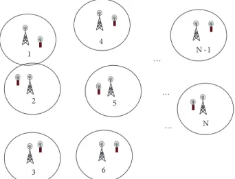
Let us consider a wireless network with N base stations (BSs) as shown in Figure 1. The figure shows a snapshot of the network with N mobile stations (MSs). For downlink transmission, the transmitter is the BS and receiver is the MS. In uplink, it is vice versa. In this paper, without loss of generality, downlink transmission is considered. Let us define link gain from BS j to MS i as gij, modelled as follows (see [19]):
gij=
sijcij
dβij , i, j = 1, 2,· · · , N, (1)
where sij is the shadow fading term, dij is the distance between the transmitter in cell j to the receiver in cell i , dβij is propagation loss with path-loss exponent β , and cij is the multipath fading factor. For further information about modelling of radio wave propagation, see, e.g., [19].
1 3 N -1 6 5 4 2 N … … …
Figure 1. A wireless network with N BSs and N co-channel MSs.
In this paper, we focus on 2-channel case because the global solution for the 2-channel case is not known as it is an NP-complete problem (e.g., [1], [3], p. 359). Furthermore, if the number of channels is different than 2, then the same algorithm can be iteratively repeated to find the solution, as explained in [3]. For example, the bisecting k -means algorithm [20] and its variants like those in [21] are such algorithms that determine the cluster to be further bisected in the next step according to various criteria defined.
Using the link gains in Eq. (1), we define the interfering link-gain system matrix as G=[ gij] where
gii = 0 , i = 1,2,..,N. The interfering link-gain system matrix G is naturally asymmetric due to the random BS and MS locations, as shown in Figure 1. Considering the 2-channel case, the channel allocation is modeled as shown in Figure 2. Given the interfering link-gain system matrix G=[ gij], an optimized channel allocation procedure assigns each of N MSs into 1 of the 2 channels according to a criterion, which would minimize the network interference. Link gain matrix and indices of MSs (1, 2, …, N -1, N) Channel 1 Indices of MSs in channel 1 (e.g. 1, 3, …, N-1) Channel Allocation Channel 2 Indices of MSs in channel 2 (e.g. 2, 4, …, N) ] [gij = G
Figure 2. Channel allocation procedure for 2-channel case.
In our formulation, without loss of generality and for the sake of brevity, we assume that the transmit powers are fixed. Once allocation of N MSs to L = 2 channels is performed, then total co-channel network interference, denoted as Intw
tot , is given by:
Itotntw= 2 ∑ s∈1 IS = ptx 2 ∑ s=1 NS ∑ j∈CS NS ∑ i∈CS (i̸=j) gij, (2)
where ptx is the BS’s fixed transmit power, CS represents the set of MSs assigned to channel/frequency s , NS is the length of the set CS (i.e. the number of MSs in channel s) , gij represents the corresponding link gains,
IS is the sum of the interferences experienced by those MSs using the same channel s , and N1+ N2= N . We
formulate the channel allocation problem as determining the sets C1 and C2 to minimize the total co-channel
network interference Intw
tot in Eq. (2)
min
determineC1andC2
Itotntw (3)
3. HNN-based solution for channel allocation problem
Before presenting the main theorem of the paper, we recall the definition of the terms ‘cut’ and ‘volume’ from graph theory:
Definition Cut of a graph: Let Gr = (V, E) denote a weighted graph, where V is set of nodes and E
represents the set of edges. In graph theory, a cut means a partition of the nodes of the graph into 2 sets; the size of the cut is the sum of the edges with a vertex on either side of the partition.
Definition maxCut of a graph: The maxCut is the cut whose size is not smaller than the size of any other cut.
Definition Volume (vol) of a set: Volume (vol ) of a set is equal to the sum of all the edges whose nodes are in the same set.
Now we are ready to present the main theorem:
Theorem Given an asymmetric interfering link-gain system matrix G (where gii = 0) , if the weight matrix
of the continuous-time HNN denoted as W is chosen as
W = D− ¯G, (4) where ¯G = 0.5(G + GT) and D = [d mn] = N ∑ j=1,(j̸=i) ¯ gij, ifm = n 0, otherwise
, then the HNN minimizes the total
co-channel network interference in Eq. (2).
Proof As in [6], we turn the channel allocation problem into a graph partitioning problem. The entry-wise 1-norm of the interfering link-gain system matrix G is equal to
∥G∥1= N ∑ i=1 N ∑ j=1 gij. (5)
Note that because matrix G consists of interfering link-gains, own-link gains are excluded, i.e. gii = 0 in Eq. (5). Because the BS’s transmit power ptx is fixed, we could ‘embed’ it into gij just for the sake of brevity. Then, considering the grouping of BSs into 2 groups C1 and C2, we write
∥G∥1= N1 ∑ i∈C1 N1 ∑ j∈C1 gij+ N1 ∑ i∈C1 N2 ∑ j∈C2 gij+ N2 ∑ i∈C2 N2 ∑ j∈C2 gij+ N2 ∑ i∈C2 N1 ∑ j∈C1 gij. (6)
Since ¯G = 0.5(G + GT) , Eq. (6) can be written as ∥G∥1= ¯G 1= N1 ∑ i∈C1 N1 ∑ j∈C1 ¯ gij+ N1 ∑ i∈C1 N2 ∑ j∈C2 ¯ gij+ N2 ∑ i∈C2 N2 ∑ j∈C2 ¯ gij+ N2 ∑ i∈C2 N1 ∑ j∈C1 ¯ gij, (7)
where ¯gij = 0.5(gij+ gji) . Because matrix ¯G is symmetric, N1 ∑ i∈C1 N2 ∑ j∈C2 ¯ gij = N2 ∑ i∈C2 N1 ∑ j∈C1 ¯
gij, and thus we can write
N1 ∑ i∈C1 N2 ∑ j∈C2 gij+ N2 ∑ i∈C2 N1 ∑ j∈C1 gij = 2 N1 ∑ i∈C1 N2 ∑ j∈C2 ¯ gij = 2 N2 ∑ i∈C2 N1 ∑ j∈C1 ¯ gij. (8)
From Eqs. (6)–(8), we can write
∥G∥1= ¯G 1= constant = I1+ I2+ J, (9) where I1= N1 ∑ i∈C1 N1 ∑ j∈C1 gij= N1 ∑ i∈C1 N1 ∑ j∈C1 ¯ gij and I2= N2 ∑ i∈C2 N2 ∑ j∈C2 gij = N2 ∑ i∈C2 N2 ∑ j∈C2 ¯
gij is the total co-channel interference for channels 1 and 2, respectively; and
J = N1 ∑ i∈C1 N2 ∑ j∈C2 gij+ N2 ∑ i∈C2 N1 ∑ j∈C1 gij = 2 N1 ∑ i∈C1 N2 ∑ j∈C2 ¯ gij, (10)
where J represents the total interference, which is eliminated once C1 and C2 are determined by the channel
allocation process.
Now let us consider the weighted graph represented by the symmetric matrix ¯G . Using the definitions of cut and the vol above from graph theory (see, e.g., [22] and [3]), Eq. (7) can be written as
vol(G) = vol(C1) + cut(C1, C2) + vol(C2) + cut(C2, C1), (11)
where vol(C1) = I1, vol(C2) = I2, and cut(C1, C2) = cut(C2, C1) = J . Thus, from Eqs. (2), (9), (10), and
(11), ∥G∥1= I ntw tot + 2cut(C1, C2). (12) From Eq. (10): min{Intw tot } = minC1,C2{I1+ I2} ≡ maxC1,C2{cut(C1, C2)} . (13)
From Eq. (14), we conclude that minimizing the total network co-channel interference is equal to the weighted
maxCut of the graph represented by symmetric matrix ¯G .
Let us define a discrete-value vector x = [ x1· · · xN] such that xi ∈ {−1, + 1}. Let C1 and C2 be the
sets of those indices i such that xi=−1 and xi= +1 Then, by definition, the cut of the graph can be written as cut(C1, C2) = N1 ∑ i∈C1 N2 ∑ j∈C2 ¯ gij= 1 2 N ∑ i=1 N ∑ j=1 ¯ gij(xi− xj) 2 . (14)
Because xi∈ {−1, + 1}, we have (xi− xj)
2
= 2(x2i − xixj )
. Using this in Eq. (14) gives
cut(C1, C2) = N ∑ i=1 ∑N j=1 ¯ gij x2 i− N ∑ i=1 N ∑ j=1 ¯ gijxixj. (15) Defining dii= N ∑ j=1 ¯
gij in Eq. (15), we can write
cut(C1, C2) = N ∑ i=1 diix2i− N ∑ i=1 N ∑ j=1 ¯ gijxixj. (16)
Rewriting Eq. (16) in matrix form gives
cut(C1, C2) = xT(D− G) x, (17)
where D = diag( dn, n = 1,. . . ,N ) is a diagonal matrix containing the row sums of G, dii= N ∑ j=1
¯
gij. From Eq. (12) and Eq. (17), and using min{Intw
tot } = max {−Itotntw}, we conclude that
min{Itotntw} = min{−xT(D− ¯G)x}. (18) On the other hand, it is well known that the Lyapunov (energy) function of the continuous-time HNN with ‘high gain’ is
V (x(t)) = −1
2f
T(x)Wf (x)− dTf (x), (19)
where x∈ ℜN×1, W∈ ℜN×N is the weight matrix of the HNN, d∈ ℜN×1, and f (x) = [f (x1)f (x2)· · · f(xN)] T
, in which f (xi) = 1− (2/(1 + e−σxi)) , σ > 0 , is a sigmoid function ( i = 1, 2,· · · , N). For a detailed analysis of the Hopfield energy function, see, e.g. [9], among others. From Eqs. (18) and (19), setting d = 0, we conclude that if the weight matrix of the continuous-time HNN denoted as W is chosen as
W = D− ¯G, (20) where ¯G = 0.5(G + GT) and D = [d mn] = N ∑ j=1,(j̸=i) ¯ gij, ifm = n 0, otherwise
, then the HNN minimizes the total
co-channel network interference in Eq. (2). This completes the proof. 2
Using the results in the theorem above, we present a novel HNN-based solution for the channel allocation problem as follows:
1) Obtain the weight matrix W in Eq. (20) (a central BS collects the measured interference power information from other BSs and obtains the matrix ¯G) .
2) Set the weight matrix of the continuous-time HNN as the matrix W in eq. (20) and set d = 0. 3) Let the continuous-time HNN evolve by time and determine the channel allocations according to the outputs of the HNN.
4. Simulation results
As benchmarks we choose a minimum-interference-channel allocation algorithm due to its wide use in practice and its high performance in random BS locations scenarios, and spectral clustering-based algorithms [6] due to their high performance in symmetrical BS locations scenarios and effectiveness in the maxCut graph partitioning problem. As a minimum-interference algorithm, we chose the basic greedy asynchronous distributed interference avoidance algorithm (GADIA) from [5].
In our simulations, we examine a radio system borrowed from [6], which is a direct-sequence code division multiple access system. The link gains are modelled by Eq. (1). In the parameter setting, the path-loss exponent
β = 3 and the shadow fading term sij are produced by a log-normal distribution whose variance is 4 dB, as in the radio network in, e.g., [6].
Dynamic equations of the continuous-time HNN with N states are given as ˙
x =−Ax + Wf(x) + Bu + d
y = f (x) , (21)
where x ∈ ℜN×1 is the state vector, A ∈ ℜN×N is the diagonal self-feedback matrix, W ∈ ℜN×N is the weight matrix, B∈ ℜN×M is the input-weight matrix, u∈ ℜM×1 is the input vector, y∈ ℜN×1 is the output vector d∈ ℜN×1 is a constant, and f (x) = [f (x1)f (x2)· · · f(xN)]
T
, in which f (xi) = k (−1 + (2/(1 + e−σxi))) ,
kj, σj > 0 , is a sigmoid function ( i = 1, 2,· · · , N). From the theorem above, the weight matrix W is chosen according to Eq. (20). Comparing Eq. (18) with Eq. (19), we set B=0 and d = 0.
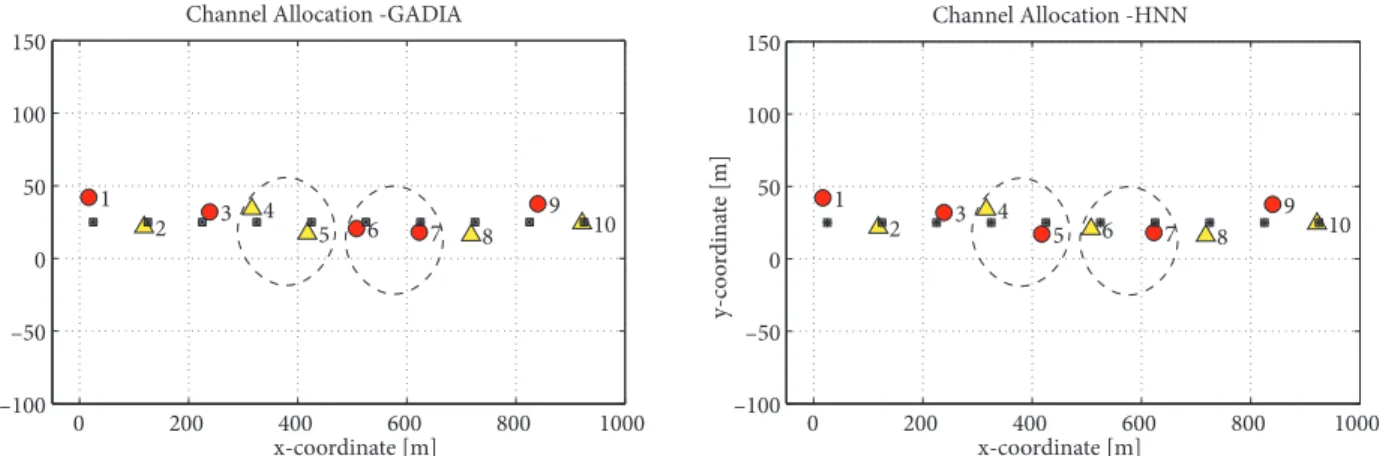
Example 1 In this illustrative example, there are 10 BSs located on a straight line as shown in Figure
3. BS locations are indicated as stars in squares, and mobile locations are shown as triangles. The channel allocation results of the basic GADIA [5] and the proposed method are also indicated in Figure 3a and Figure 3b, respectively. 0 200 400 600 800 1000 –100 –50 0 50 100 150 1 2 3 4 5 6 7 8 9 10 x-coordinate [m] y-co o rdin at e [m]
Channel Allocation -GADIA
0 200 400 600 800 1000 –100 –50 0 50 100 150 1 2 3 4 5 6 7 8 9 10 x-coordinate [m] y-co o rdin at e [m] Channel Allocation -HNN
Figure 3. A snapshot of the 1-dimensional network in Example 1 with 10 BSs. The center BS locations are shown as stars in squares, and the circles and triangles (in different gray levels) indicate the MS locations with their channel allocations by (a) basic GADIA [5] and (b) the proposed HNN-based solution.
The circles and triangles (in different gray levels) indicate the MS locations with their channel allocations. The triangle and circle represent channels 1 and 2, respectively. As seen from Figure 3a, mobiles 4 and 5 (as well as mobiles 6 and 7), which are next to each other, are allocated into the same channel, which would deteriorate
the performance. On the other hand, the proposed HNN-based solution gives the globally optimum solution for this scenario, as seen in Figure 3b. The spectral clustering also gives the same result as the proposed HNN in this example. The average signal-to-interference + noise ratio (SINR) per mobile station by the proposed solution in Figure 3b is 4.85 dB higher than that of the reference algorithm (i.e. basic GADIA-type minimum interference algorithm) in Figure 3a. This corresponds to an average (Shannon) channel capacity increase of 2.5484 [bits/Hz] by the proposed algorithm.
Evolution of the states of the proposed continuous-time HNN whose weight matrix is equal to the weight matrix in Eq. (20) is shown in Figure 4. Note that Figure 4a shows the states, not the output, of the neurons. The outputs of the neurons are saturated to (–1, +1) due to the sigmoid function. The evolution of the Lyapunov (energy) function with respect to normalized time is shown in Figure 4b. As can be seen, the energy function decreases by time as converging to an optimized solution.
0 2 4 6 8 –2 –1 0 1 2 1 2 3 4 5 6 7 8 9 10 time [s] x (t)
Evolution of states with time for HNN
0 0.5 1 1.5 2 2.5 –10 –8 –6 –4 –2 0
Lyapunov function V(t) for HNN
L ya p un o v f un ct io n V(t) time [s]
Figure 4. (a) Evolution of the states of the proposed continuous-time HNN whose weight matrix is equal to the weight matrix in Eq. (20) in Example 1 and (b) corresponding Lyapunov function in Eq. (19).
In order to compare the average performance of the proposed algorithm as compared to the reference algorithm for this one-dimensional scenario, we examine 1000 snapshots. At each snapshot, the locations of the MSs are randomly determined while the BSs’ locations are fixed. Average relative SINR in dB and corresponding relative channel capacity with respect to that of the reference case (i.e. minimum interference allocation algorithm) over 1000 independent snapshots are presented in Table 1. The proposed algorithm outperforms the reference algorithm, and the best performance is obtained by the spectral clustering for this particular 1-dimensional symmetric BS-location scenario.
Table 1. Relative average SINR gains in dB and corresponding average channel capacity [bits/Hz] with respect to that of the reference case (minimum interference allocation algorithm) in Example 2 over 1000 snapshots.
N (# of BSs)
Relative
Relative avg. channel capacity [bits/Hz] SINR [dB]
Spectral clust. Proposed HNN Spectral clust. Proposed HNN
10 (1-dimensional) +2.8658 +2.0695 +1.9508 +1.6180
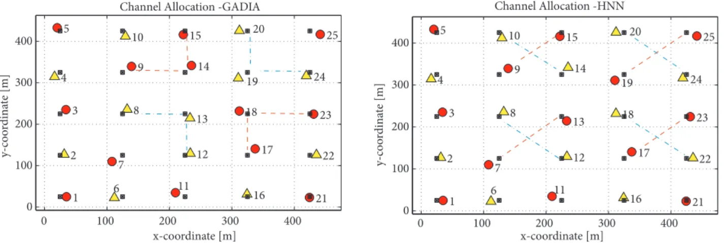
Example 2 In Example 1 above, the center MSs are located on a straight line (in 1 dimension). In this illustrative example, the cellular radio system is in 2 dimensions, and there are 25 BSs located on a 5-by-5
grid as shown in Figure 5. The channel allocation results are also given in Figure 5a and Figure 5b for the basic GADIA [5] and the proposed method, respectively. Comparing the channel allocations of mobiles 9-14-15, 8-12-13, 17-18-23, and 19-20-24, the basic GADIA-like minimum interference algorithm gets stuck at a local minima, while the proposed HNN finds the globally optimum solution. The spectral clustering also gives the same result as the proposed HNN in this example. The average SINR by the proposed solution in Figure 5b is 1.2697 dB higher than that of the reference algorithm (basic GADIA-type minimum interference algorithm) in Figure 5a. This corresponds to an average (Shannon) channel capacity increase of 1.1825 [bits/Hz] by the proposed algorithm. 0 100 200 300 400 0 100 200 300 400 1 2 3 4 5 6 7 8 9 10 11 12 13 14 15 16 17 18 19 20 21 22 23 24 25 x-coordinate [m] y-co o rdin at e [m]
Channel Allocation -GADIA
0 100 200 300 400 0 100 200 300 400 1 2 3 4 5 6 7 8 9 10 11 12 13 14 15 16 17 18 19 20 21 22 23 24 25 x-coordinate [m] y-co o rdin at e [m] Channel Allocation -HNN
Figure 5. A snapshot of the 2-dimensional network in Example 2 with 25 BSs. The BS locations are shown as stars in squares, and the circles and triangles (in different gray levels) indicate the MS locations with their channel allocations by (a) basic GADIA [5] and (b) proposed HNN-based solution.
Average relative SINR in dB and corresponding relative channel capacity with respect to that of the reference case (i.e. minimum interference allocation algorithm) over 1000 independent snapshots are presented in Table 2. The proposed algorithm outperforms the reference algorithm and the spectral clustering for this particular 2-dimensional symmetric BS-location scenario.
Table 2. Relative average SINR gains in dB and corresponding average channel capacity [bits/Hz] with respect to that of the reference case (minimum interference allocation algorithm) in Example 2 over 1000 snapshots.
N (# of BSs)
Relative
Relative avg. channel capacity [bits/Hz] SINR [dB]
Spectral clust. Proposed HNN Spectral clust. Proposed HNN
25 (2-dimensional) +0.0959 +0.3141 +0.1321 +0.3941
All the simulation results above confirm the effectiveness of the proposed algorithm. The key reason for the good performance of the proposed algorithm comes from the theorem above. Comparing Eqs. (1), (18), and (19), the proposed HNN minimizes the total co-channel network interference in Eq. (2).
Example 3 In all the examples above, the BSs locations are located ‘symmetrically’ with respect to a point or a line. In this example, the BS locations are fully random. We examine different sizes of cellular networks ( N = 6 to 24). The area of simulation scenario is 50N [m] by 50N [m], where N is the number of BSs. The average results are obtained over 1000 random snapshots. The average SINRs in dB and the average (Shannon)
channel capacity in bits/Hz normalized with respect to that of the basic GADIA case are shown in Table 3. The proposed HNN-based method outperforms both the basic GADIA-type minimum interference algorithm and the spectral clustering method for random BS locations for middle-size wireless networks ( N = 6 to 24). Table 3. Average SINR gains in dB and average channel capacity [bits/Hz] with respect to that of the reference case (minimum interference allocation algorithm) in Example 3.
SINR [dB] Average channel capacity [bits/Hz]
N (# of BSs)
Spectral clust. Proposed HNN Spectral clust. Proposed HNN
10 –2.36 +0.63 –1.74 +0.71
14 –4.01 +0.43 –2.32 +0.52
18 –3.92 +0.57 –2.29 +0.65
24 –3.59 +0.62 –2.19 +0.70
5. Conclusions
In this paper, we first turn the channel allocation problem in wireless systems into a maxCut graph partition-ing problem. Based on the correspondpartition-ing formulation, we then propose and analyze a simple and effective continuous-time HNN-based solution by determining its symmetric weight matrix from the asymmetric link-gain-system matrix (or received-signal-power-system matrix) of the radio network.
Computer simulations for 1-dimensional and 2-dimensional middle-size ( N = 10 to 25) cellular radio systems, where the aim is to minimize the total network interference, show that that the proposed HNN-based solution outperforms the reference algorithm (i.e. the standard minimum-interference-HNN-based channel allocation algorithm) in all cases. Furthermore, the average simulation results also show that the proposed algorithm outperforms the spectral clustering method for symmetrical BS locations scenarios as the number of BSs increases ( > 20), and for all asymmetrical BS locations scenarios for any number of BSs.
References
[1] L. Narayanan, “Channel assignment and graph multicoloring”, in Handbook of Wireless Networks and Mobile Computing (I. Stojmenovic, editor), Hoboken, NJ, USA, Wiley, pp. 71–94, 2002.
[2] I. Katzela, M. Naghshineh, “Channel assignment schemes for cellular mobile telecommunication systems: a com-prehensive survey”, IEEE Communications, Surveys & Tutorials, Vol. 3, pp. 10–31, 2000.
[3] M.E.J. Newman, Networks: An Introduction, Oxford, UK, Oxford University Press, 2011.
[4] S. Chieochan, E. Hossain, J. Diamond, “Channel assignment schemes for infrastructure-based 802.11 WLANs: a survey”, IEEE Communications, Surveys & Tutorials, Vol. 12, pp. 124–136, 2010.
[5] B. Babadi, V. Tarokh, “GADIA: A Greedy Asynchronous Distributed Interference Avoidance Algorithm”, IEEE Transactions on Information Theory, Vol. 56, pp. 6228–6252, 2010.
[6] Z. Uykan, “Spectral based solutions for (near) optimum channel/frequency allocation”, Proceedings of IWSSIP 2011 (18th International Conference on Systems, Signals and Image Processing), Sarajevo, Bosnia and Herzegovina, 2011. [7] J.J. Hopfield, “Neural networks and physical systems with emergent collective computational abilities”, Proceedings
of the National Academy of Sciences of the USA, Vol. 79, pp. 2554–2558, 1982.
[8] J.J. Hopfield, D.W Tank, “Neural computation of decisions in optimization problems”, Biological Cybernetics, Vol. 52, pp. 141–146, 1985.
[10] O. Lazaro, D. Girma, “Real-time operational aspects of Hopfield neural network based dynamic channel allocation scheme”, Electronics Letters, Vol. 40, pp. 1141–1143, 2004.
[11] C.W. Ahn, R.S. Ramakrishna, “QoS provisioning dynamic connection-admission control for multimedia wireless networks using Hopfield neural networks”, IEEE Transactions on Vehicular Technology, Vol. 53, pp. 106–117, 2004. [12] D. Calabuig, J.F. Monserrat, D.G. Barquero, O. Lazaro, “User bandwidth usage-driven HNN neuron excitation method for maximum resource utilization within packet-switched communication networks”, IEEE Communication Letters, Vol. 10, pp. 766–768, 2006.
[13] M. Sheikhan, E. Hemmati,“High reliable disjoint path set selection in mobile ad-hoc network using Hopfield neural network”, IET Communications, Vol. 5, pp. 1566–1576, 2011.
[14] I. Zabalawi, A. Jaradat, R. Al-Khawaldeh, “A dynamic channel assignment technique based on the discrete Hopfield neural network model”, Proceedings of the Fifth International Symposium on Signal Processing and Its Applications, Vol. 2, pp. 673–676, 1999.
[15] J.S. Kim, S.H.P. Park, P.W. Dowd, N.M. Nasrabadi, “Cellular radio channel assignment using a modified Hopfield network”, IEEE Transactions on Vehicular Technology, Vol. 46, pp. 957–967, 1997.
[16] K. Smith, M. Palaniswami, “Static and dynamic channel assignment using neural networks”, IEEE Journal on Selected Areas in Communications, Vol. 15, pp. 238–249, 1997.
[17] N.A. El-Fishawy, M.M. Hadhood, S. Elnoubi, W. El-Sersy, “A modified Hopfield neural network algorithm for cellular radio channel assignment”, Proceedings of IEEE-VTS Fall VTC 2000, Vol. 3, pp. 1128–1133, 2000. [18] H. Lee, C.C. Tuan, T.P. Hong, “A maximum channel reuse scheme with Hopfield Neural Network based static
cellular radio channel allocation systems”, Proceedings of IJCNN 2008 (International Joint Conference on Neural Networks), pp. 3660–3667, 2008.
[19] T.S. Rappaport, Wireless Communications: Principles & Practice, 2nd ed., Upper Saddle River, NJ, USA, Prentice Hall, 2002.
[20] S.M. Savares, D. Boley, “On the performance of bisecting k-means and PDDP”, Proceedings of the 1st SIAM International Conference on Data Mining, pp. 1–14, 2001.
[21] R. Kashef, M.S. Kamel, “Enhanced bisecting k -means clustering using intermediate cooperation”, Pattern Recog-nition, Vol. 42, pp. 2557–2569, 2009.
[22] U.V. Luxburg, A Tutorial on Spectral Clustering, Technical Report TR-149, T¨ubingen, Germany, Max-Planck Institute for Biological Cybernetics, 2006.