щ і · ^ « 5 5 — ıS » i « T * j«~ * î* -U "'« -4^··^ M . 4 ■«•■^S^-<U., « · * ^ m - J J : ■| Г. ;· · ;!5
нь
İ891.9J
\ЧЧЪ
"■ " T·' "' ■’'■ ' ■ ■, ·■’1*«^. '* te» ·■' ,«' . ; ‘n it: ' **í; / ' - “ гѵгч /Иг> 'f * У.І * . <¡ ■■ - í · ' Λς . Й-іЦ'· Λ - - / β .■τ: , ^ 'ί- ··* * rt^. ο ·( Λϊί; ^ ^ . ^ ■ . ^ , - ^ r j¡c4 . ^.,. ( ^ ΐ £2 :,,(^ ·> .4·· ^ 4^ » '^ .· . к. ’ >■* «τι —,Γ, i ' J V -· . . ,^/V ■ Τ' · * : - 'μ» ■ / л r> * . /г. /“ <Г · - * /t, ' ·1 ’■ '<*iM¿<'' «dit. <»' ^ ^ ..AN APPLICATION OF AN ENTROPY APPROACH TO THE TURKISH MANUFACTURING INDUSTRY
A Thesis
Submitted to the Department of Economics and the Institute of Economics and Social Sciences
of Bilkent University
In Partial Fulfillment of the Requirements for the Degree of
MASTER OF ARTS IN ECONOMICS
by
Şule ALTABAN October, 1993
нь
-
¿
I certify that I have read this thesis and in my opinion it is fully adequate, in scope and in quality, as a thesis for the degree of Master of Arts in Economics.
I certify that I have read this thesis and in my opinion it is fully adequate, in scope and in quality, as a thesis for the degree of Master of Arts in Economics.
Asst.Prof.Dr.Erol ÇAKMAK
I certify that I have read this thesis and in my opinion it is fully adequate, in scope and in quality, as a thesis for the degree of Master of Arts in Economics.
iL·
Asst.Prof. Dr.Faruk SELÇUK
ABSTRACT
AN APPLICATION OF AN ENTROPY APPROACH TO THE TURKISH MANUFACTURING INDUSTRY
Şule ALTABAN MA in Economics
Supervisor: Prof.Dr.Orhan GÜVENEN November 1993, 70 pages
This study concerns an application of concentration measurement for the Turkish Manufacturing Industry using information theory. Theil's (1971) disaggregation of entropy is converted to handle the whole
manufacturing industry in order to see the competitive and
monopolistic trends. The between-group variation and within-group variation values are computed for three yearly period between 1989 and 1991 using sales figures. These values give the intersectoral and inter-firm differentiations for the manufacturing industry. The study concludes that the distribution for sales figures within the sector
displays a less equal pattern than the intersectoral analysis,
although the general relative entropy values shows only a tendency to equal shares for the Turkish Manufacturing Industry.
Keywords: Concentration, information theory, entropy, between-group
variation, within-group variation, intersectoral
differentiation, inter-firm differention, relative entropy.
ÖZET
BİR ENTROPİ YAKLAŞIMININ
TÜRK İm a l a t s a nayii IçIn bIr u y g u l a m a s i
Şule ALTABAN
Yüksek Lisans Tezi, iktisat Bölümü Tez Yöneticisi: Prof.Dr.Orhan GÜVENEN
Kasım 1993, 70 sayfa
Bu çalışmada, bilgi teorisi kullanılarak Türk imalat Sanayiinin
yoğunlaşma ölçümünün bir uygulaması yapılmıştır. Theil'in (1971)
entropi ayrıştırması, rekabetçi ve tekelci eğilimleri görmek üzere, bütün imalat sanayiini kapsayacak şekilde uyarlanmıştır. 1989 ve 1991 yıllarını kapsayan üç yıllık dönem için, satış rakamları kullanılarak
gruplar arası varyasyon ve grup içi varyasyon değerleri
hesaplanmıştır. Bu değerler imalat sanayii için sektörler arası ve
firmalar arası farklılaşmayı vermektedir. Çalışmamızda, göreli
entropi değerlerinin Türk imalat Sanayii için yalnızca eşit genel paylar yönünde bir eğilim göstermesine karşın, sektör içi satış rakamları dağılımının sektörler arası analize göre daha eşitsiz bir model gösterdiği sonucuna varılmıştır.
Anahtar Sözcükler: Yoğunlaşma, bilgi teorisi, entropi, gruplar arası
varyasyon, grupiçi varyasyon, sektörler arası
farklılaşma, firmalar arası farklılaşma, göreli entropi.
ACKNOWLEDGEMENTS
I am grateful to Prof.Dr.Orhan Güvenen for his close
supervision and guidance throughout the study. Without his generous contributions, this study would surely not see the 1ight of the day.
I would like to extend my special thanks to Dr.Murat Güvenç for his help in.project formulation and also for his patient assistance at every stage of the study.
I am particulary indebted to Emine Koçberber, Merih Güneş and Münür Yayla for their invaluable help in collecting data.
I owe a lot to Ayşegül Altaban for her help in editing the final draft.
My special thanks are due to Zeliha Sözüpişkin and Alper Yılmaz for their help in typing.
I also thank to my mother and my father for their understanding and patiance during my troubled times.
Last but not the least, I would like to extend my gratitude to Asst.Prof.Dr.Erol Çakmak and Asst.Prof.Dr.Faruk Selçuk for their support and understanding during my final presentation.
TABLE OF CONTENTS
ABSTRACT... iii
SUMMARY... iv
ACKNOWLEDGEMENTS... v
LIST OF TABLES... vii
LIST OF FIGURES... viii
CHAPTER 1. INTRODUCTION... 1
CHAPTER 2. A GENERAL OUTLOOK TO THE MEASURES OF INDUSTRIAL CONCENTRATION... 2
2.1. The Concentration Concept... 2
2.2. Factors Affecting Concentration... 6
2.3. Some Measures of Concentration... 7
2.3.1. The Concentration Ratio... 7
2.3.2. The H-Index (Hirshman-Herfindahl Index)___ 9 2.3.3. Entropy Index... 11
2.3.4. Measures of Variation... 11
2.3.5. The Concentration Curve... 13
2.3.6. The Lorenz Curve... 15
2.3.7. The Gini Coefficient... 17
2.4. More on Concentration As a Criterion of Market Structure... 18
CHAPTER 3. INFORMATION THEORY AND ENTROPY... 20
3.1. The Information Concept... 20
3.2. Entropy of a Random Variable... 22
3.3. Some Properties of H(x) As a Measure of Uncertainty... 24
3.4. Entropy as a Measure of the Degree of Competition in Economic Theory... 25
3.5. Relative Entropy... 28
CHAPTER 4. AN APPLICATION OF AN ENTROPY APPROACH TO THE TURKISH MANUFACTURING INDUSTRY... 31
4.1. Disaggregation of the Entropy... 31
4.2. Description of the Data... 33
4.3. Results of the Analysis... 34
CHAPTER 5. CONCLUSION... 43
REFERENCES... 45
APPENDIX A. ENTROPY ANALYSIS FOR 1989, 1990 AND 1991... 47
APPENDIX B. INTERNATIONAL STANDARD INDUSTRIAL CLASSIFICATION... 68
1. Disaggregated Entropy Values... 34
2. Sales, Number of Sectors and Firms for 1989-1991... 35
3. Relative Entropy... 35
4. Redundancy and Relative Entropy... 38
5. Total Sales and Pb Values for Petroleum Refineries ... 39
6. An Entropy Analysis for the Sector 3530 in 1989, 1990 and 1991... 40
LIST OF TABLES
Table Page
1. The Concentration Curve... 13 2. Lorenz Curve... 16 3. Entropy in nats... 23 4. Entropy in bits... 23 LIST OF FIGURES Figure Page
CHAPTER 1. INTRODUCTION
In this study, the concentration trends in Turkish Manufacturing Industry are analyzed with an information theoretic perspective.
Theil's (1971) disaggregation of entropy measure is firstly converted to handle the whole Turkish Manufacturing Industry and then applied to a set of 3-year data pertaining to years 1989-1991. Yet, the study is mainly empirical in nature and does not involve a theoretical approach.
The most recent study which shed light to this study in literature is Erlat (1975), which applies various concentration measures to the Turkish Manufacturing Industry.
In Chapter 2, an explanation of the concentration concept is provided together with an overview of the relevant measures given in the 1iterature.
In Chapter 3, information theory is overviewed and entropy, as a
measure of the degree of competition in economic theory, is
explained. :
In Chapter 4, Theil's (1971) disaggregation of entropy is applied to
the Turkish manufacturing industry and the competitive and
monopolistic trends are discussed according to the computational results. The underlying rationale of Theil's disaggregation is found
in the decomposition of total information expectation into the
between group information expectation and a weighted average of the within group information expectations.
CHAPTER 2. A GENERAL OUTLOOK TO THE MEASURES OF INDUSTRIAL CONCENTRATION
2.1. THE CONCENTRATION CONCEPT
Concentration is defined as the control of a small percentage of units over a large percentage of economic resources and activities. Concentration is used to measure the inequalities between firms which
constitute an economy or an industry just like measuring the
distribution pattern of income and property amongst members of
society. In other words, concentration is the state of a number of firms' controlling the economy or a certain industry. It is only via concentration concept that we can study and evaluate the extent to which the economy or a certain industry are controlled by a certain number of firms.
Concentration is usually one of the outstanding indicators of firm behaviour like production, prices, the market performance, and market structure. For example, there will be certain consequences of a high level of concentration (a certain number of firms controlling a
certain industry) in an economic structure. The most striking
consequence is an increase in monopolization trends in the structure, and moving away from a competitive status in the economy.
A market (or a unit) is said to be more concentrated than another if the number of firms operating in an economic structure decreases or the differences between the relative sizes of these units increase.
One of the significant points about concentration is as follows:
The state of a certain number of firms of a certain size controlling the economy is different from the state of a small number of firms.
having larger sizes controlling the economy. In the former case, the firms having a certain influence in the economy and a certain degree
of control are considered. This is a kind of "aggregate
concentration". It is also called the overall concentration. In the latter case, the inequality is arising in the field of activity of firms manufacturing the same goods in a certain industry. This type of concentration is called "market concentration".
According to Utton (1970) [1], several important consequences can result from concentration in economic theory. First, it will be difficult to realize an optimum allocation of resources. Utton states that, in such industries, the price of the product falls as output expands and, in equilibrium, price will be in excess of marginal cost. In such cases, there will be a lack of competition. In an industry of high concentration, prices will be higher and output will be lower, compared with a competitive industry. Secondly, according to Utton, lack of competition in highly concentrated industries affect the internal efficiency of firms. In a perfectly competitive market, firms try to maximize their profits, as their inefficiency can cause their elimination from the market. On the other hand, Utton say’s, in monopolistic and oligopolistic markets, firms do not have such a sharp incentive. Their inefficiency brings different results
from their being in a perfect competition. In monopolistic (or
oligopolistic) cases, their inefficiency will result in a reduction in their profits.
[1] Utton, M.A. (1970). Industrial Concentration. Middlesex,England; Penguin Books. Books, pp.l4.
"In addition to the misallocation of resources between industries that occurs as a result of high concentration, therefore, a further misallocation may take place within firms because of their failure to maximize profits" [2]. Thirdly, there can be a change in the distribution of income due to concentration in an economy. This is mainly because a greater share of income goes to the concentrated industries as there become sharp differences in the profit rates between industries in the economy. "The excess profits are due to the protected position of the firms and they do not fulfill the economic function of in ducing increased investment in the industry from new firms" [3].
It is easy to realize that all these three effects stated by Litton, are related with the market concentration. At this point, it is again important to distinguish "market concentration" from "overall concentration".
Via overall concentration (aggregate concentration) is aimed a
certain measurement for outstanding firms, having major influence in a country's economy. This is achieved by the evaluation of a ranking of firms according to their total sales, total assets, total number of employees or according to the net profits. This approach yields the level of importance of large firms' influence in economy.
On the other hand, market concentration, aids in the comparison of firms operating in an industry in terms of their capacities, sizes, their shares and various indicators, considering the total number of firms simultaneously. Thus, if in an industry, a certain number of
[2] Litton, op.cit., pp.l5 [3] Litton, loc.cit.
firms have a dominance with respect to some pre-determined indicators, there is said to be more concentration in that industry.
"For example, if 7 firms are operating in textile industry in a country, and if one firm has 50% share and a second firm has 25% share and the rest has 25% share in the market, it could be said that there is a high degree of concentration in this industry" [4].
Yet, concentration is not a simple arithmetic interpretation made with respect to the idea "if a small number of firms are operating within an industry, we can talk about concentration". According to Akoğlu (1976), this fact can be clarified with the following example
[5]:
Assume that 123 firms are operating in the aformentioned textile
sector. At first glance, it could be said that there is no
concentration in that industry. Yet, this result is deceiving with regard to the number of firms. Since, if the relative sizes of the firms are considered, the interpretation will change. According to Akoğlu (1976), assume that the firm with the largest capacity has 20% share, the second one has 18% share, and the third and the fourth largest firms have 12% and 10% share respectively, of the market. This could mean that 4 of the 123 firms have a control over 60% of the industry. What does this mean? In this industry, we can talk
about concentration. In economic theory, the basic aim of the
concentration concept is to clarify the existence of monopolistic trends and a monopolistic operation in an industry which seems to be competitive at first glance.
[4] Akoğlu, T. (1976). Yoğunlaşma ve Ekonomik Yapı, Devlet Yatırım Bankası, Ankara, pp.6.
The level of concentration is influenced due to some factors. According to Utton (1970), these factors can be classified according to their influences on concentration. This classification depends whether the factors improve concentration or not [6].
As noted by Utton (1970) [7], the economies of large-scale plants,
the economies of the large multi-plant firm, and research,
development and modern technology can be stated as the factors having positive effects on industrial concentration. There are also factors
having negative effects on industrial concentration. These are
barriers to new competition and the inducement to monopolize or cartelize.
At this point, the expression of "negative effect on concentration" is important. For example, one of the negative effects stated by Utton is the inducement to monopolize. In other words, these are the effects causing monopolization. Here, these effects are regarded as negative effects on concentration. What does this mean? This means, if monopolization increases beyond a level, this will bring some disadvantages.
By negative effects, we mean the effects which help to maintain a
level of concentration which is not necessarily desirable for
efficiency or for technical progress. That means, if concentration has been reached up to a certain level in an economy, some various factors (negative factors) may bring some disadvantages for this economy.
[6] Also see: Erlat, G. 11975). Measures of Industrial Concentration
with an Application to the Turkish Manufacturing Industry^
UnpubIished M.S.Ihesis, MtTU, pp.4-5. [7] Utton, op.cit., pp.19-25.
One of the main factors influencing concentration is the want to obtain high profits. Profit has usually an inverse relationship with the number of sellers (firms) operating in an industry. On the other hand, we can say that, profit has a direct relationship with the firm's size, and its expenditures on advertising.
Firms increase their profits by reducing the inter-firm competition via mergers giving rise to a smaller number of firms and a higher level of concentration. This enables the case of determining prices much higher than the real costs in an industry with a higher level of concentration.
Those type of aggreements and mergers changing the whole structure of competition gave rise to a variety of institutional organizations. These can be categorized as vertical mergers and horizontal mergers In horizontal mergers, firms within an industry merge, while in vertical mergers, firms at different stages of the production of a commodity, yet having different subjects of production, merge. In vertical and horizontal mergers, the firms' union is realized in various firms and in different institutional organizational styles. The main ones are trusts, mergers and cartels [8].
2.3. SOME MEASURES OF CONCENTRATION
2.3.1. The Concentration Ratio
Concentration ratio is one of the oldest concentration criteria. In an industry, it is defined as follows:
M
C K , =£5·, /=1
[8] See: Çelebioğlu, N. (1990). Türk İmalat Sanayiinde Tekelci
Fiyatlama D a v r a m s l a n m n Olup ÖTmadıgımn Arastinlmas-i. d
T
e"
pp.25-26.Sjis the share of the i th. firm and M is the number of largest firms in the industry.
Concentration ratio is computed as the cumulative share of M firms. In other words, concentration ratio is the total market share of the M largest firms. Thus, this ratio does not consider all firms in the industry.
"If we want to understand the evolution of the concentration process in an industry, the concentration ratios will be inadequate with respect to some aspects" [9]. The concentration ratio does not state if the largest firms are always the same ones. Thus, these ratios do not explain the changes in sizes in an industry.
At this stage, the determination of M is of interest. M is mostly selected arbitrarily. Conventionally it is taken to be 4,8 or 20. The criterion considered in selecting the firms is the sales, the level of employment or the value-added.
There are mainly two purposes of measuring the concentration ratio [
10
]:i) Measuring the share of the largest firms producing a certain commodity within an industry.
ii) Determining the relative sizes of the largest units.
Some empirical studies aiming to alleviate the subjectivity in
determining M indicate that the 50% level in analyzing 4 firms is equivalent to the 70% level in analyzing 8 firms. These studies have
[9] Tekeli, İ., S.İlkin, A.Aksoy, Y.Kepenek (1981). Türkiye'de Sanayi Kesiminde Yodunlaşma, Ekonomist Yayınevi, Ankara, pp.22.
[10] See: Thorp Icrowd^, The Structure of Industry, Washington, 1941, Part V.
also revealed that the 50-55% level in analysis of 4 firms and 70% level in analysis of 8 firms can be taken as the starting point in
concentration studies. These starting points differ as to the
regional and national production areas. For example, firms making regional production, the starting point of critical concentration is about 20% [11].
As could be seen, despite of some empirical difficulties
concentration ratio (CR) is one of the imp^ortant indicators related to market structure.
It must be added that, "the concentration ratio is a one dimensional measure, it is a decreasing function of the number of equally sized firms and also it has a range of 0 to 1" [12].
2.3.2. The H-Index (Hirshman-Herfindahl Index)
The H-Index is found as the sum of squares of market shares of all of the firms:
n
H = ' ^ S f where S¡ is the share of the i-th firm and n is the <=i number of firms [13].
Contrary to CR, the H-Index takes all the firms into account.
If a single firm exists in the industry, H-Index attains its highest value, which is 1. If all the firms have equal sizes, the index attains its lowest value, 1/n, and the index attains gradually higher values as the inequalities between firms increase.
[11] See: Tekeli, İlkin, Aksoy, Kepenek, op.cit., pp.22-23. [12] Erlat, op.cit., pp.l8.
[13] Contrary to concentration ratio, the H-index takes all the firms into account.
The H-Index is a comprehensive index since it considers the complete distribution and it is sensitive to the changes in firms' sizes and the decrease in number of firms considered.
Since the squares of Sj 's are used in computing the index, the contribution of the small firms to the H-Index is even smaller. Hence, changes in shares of small firms will not affect the value of H-Index significantly.
"The H-Index has an interesting meaning: If two units of the same industrial good at the market are randomly selected, the probability that both are produced at the same plant is equal to the value of H-
Index" [14].
Besides, according to Erlat (1975) [15], the H-Index satisfies some basic properties of any concentration measure, which are also stated by Hall-Tideman (1967).
At this point, we will briefly explain these basic properties [16]:
1) Concentration is a one dimensional phenomenon. For example, if two industries are of concern, either one of them is more concentrated
or they have equal degrees of concentration. Therefore the
concentration measure selected should reflect this situation.
2) Concentration is independent of the absolute size of the industry. Relative size is of importance. For example, if pj denotes the i- th. firm's share in the industry, concentration is a function of Pj 's.
[14] Tekeli, İlkin, Aksoy, Kepenek, op.cit., pp.23. [15] Erlat, op.cit., pp.29.
[16] See: Hall, M., and N.Tideman (1967). Measures of concentration. Journal of the American Statistical Association. Vol.62, pp.l62- 168.
3) Every measure of concentration should reflect the changes in Pj 's. For example, if one or more firms move from lower concentration levels to upper levels, the concentration value should increase, etc.
4) If an industry is subdivided into N firms of equal sizes, the concentration measure should be a decreasing function of N.
5) Concentration measure takes values between 0 and 1.
2.3.3. Entropy Index
Entropy index is an index that has its origins in information theory. Entropy is a statistical measure of information given by the pattern and frequency of a probability distribution.
Entropy index is found as the weighted sum of the logarithms of the market shares of the firms in an industry:
n
E = ■ log5,. , where
i=l
n = number of firms in the industry Sj= share of the i-th. firm.
A detailed understanding and an application of the "entropy index" is the main aim of this thesis [17].
2.3.4. Measures of Variation
These are namely the mean, standard deviation, variance, and the coefficient of variation.
[17] For this purpose, a detailed explanation of the entropy concept is given in Chapter 3.
y " X
M e a n : fi - - ' . where n=number of firms in the industry. n
Variance: <j^ =
Standard Deviation: cr =
The Coefficient of Variation: C = —
According to Tekeli, İlkin, Aksoy, Kepenek (1981) [18], the advantage of these measures over other measures is that they give information pertaining to the complete distribution and they also apply to information collected with sampling.
At this point, we need to mention the case of computation of H index using C-coefficient.
H index can also be found as follows:
H =
C - 1
n where C= Coefficient of variation
n= # of firms in the industry.
"Thus H index also has the property of computability from the information obtained from random sampling" [19].
As could be seen, H index has the property of accounting for the
firms' relative size and the absolute number of firms.
Simultaneously, H becomes a comprehensive and multi-purpose index.
[18] Tekeli, İlkin, Aksoy, Kepenek, op.cit., pp.24-25. [19] Ibid, pp.25
Cu^ulo^'/^ CDi^-iroL |?€'^C€H'V53^
CaccorTjiti3
-fo a ctr-ja\^ (^nciícα^'0^г.}.‘There are a number of indicators used in explaining the market and share distrubition, in other words in clarifying the number of firms controlling the market. These are;
- sales, - employment, - total assets, - value added.
The concentration curve is a two-dimensional plot of one of the above
indicators versus the cumulative number of firms. Thus the
objectivity of selecting the number of firms in the calculation of concentration ratio is alleviated. All the concentration ratio values can be read on the concentration curve. The following figures are two representative concentration curves [20].
c.curve A.
C· curve 4-.
2.3.5. The Concentration Curve
o 1 If 5 io <5 jio ;2.5
Figure I. The concentration curve
> CUvMulaFive
It should be noted that here the firms are ranked in descending, order of their market chares. According to C curve I, Akoglu (1976) states that if the vertical axis denotes the sales quantities of firms, C curve I indicates that 4 of the firms in this industry own [20] See: Ako^lu, op.cit., pp.54.
3) This method has a major advantage in comparison of two firms and due to the inherent structure of the index, it can be explicitly understood.
Yet Erlat also states a major disadvantage of concentration curve, the measure is not unidimensional. The concentration curves may intersect. For example, in case of two industries, the intersection points indicate the equalities of concentration of two industries.
"The intersection of concentration curves means that one may find the states which show a particular industry more or equally concentrated or less concentrated than another industry" [22].
2.3.6. The Lorenz Curve
Lorenz curve is used to reveal any inequalities in a distribution.
The plotting and application of Lorenz curve is very similar to the
concentration curve. The vertical axis shows the cumulative
percentages of a relevant economic measure of size, such as output or assets. The cumulative percentage (or, the number) of firms in the industry, from the smallest to the largest is shown on the horizontal axis [23].
As shown in the following figure, the line joining the diagonal ends is called the "line of equal distribution" (line of equality). If all of the firms have equal shares of market control, the Lorenz curve can be found as overlapping with this line. In such a case, we can no longer talk about an inequality in the distribution. In fact, the aim of Lorenz curve is to determine the amount of deviation from this
[22] Erlat, loc.cit.
line. The industry is said to be more highly concentrated the farther the Lorenz curve is from this line, hence the greater the area in between the two curves is [24].
The following pictorial example will facilitate the understanding of Lorenz curve [25]:
The determination of the total number of firms is important in plotting Lorenz curve. According to Hall and Tideman (1967), when entries to and exists from an industry occurs, the shares of the large firms do not change, yet the Lorenz curve indicate these as if big changes have recurred in the industry. Because of this fact, Erlat (1975) [26] have stated this to be a deceiving element in measuring concentration. Because, many firms which may be disregarded can, in fact, greatly influence the shape of the Lorenz curve. The
interpretation of the curve based on the drawing may thus be
unhealthy.
[24] See: Akoglu, op.cit., pp.56-57. [25] See: Akoglu, loc.cit.
[26] Erlat, op.cit., pp.25.
Gini coefficient is used to measure the area between the line of equal distribution and the Lorenz Curve.
"...this concentration coefficient is a measure of the extent to which firms in the industry are unequal in size. For this reason it is common to refer to the Gini coefficient as a measure of inequality rather than of concentration" [27]. Like the Lorenz curve, the Gini coefficient is also based on the entire distribution of firms. So changes at any point in the distribution will be recognized by both the Gini Coefficient and the Lorenz Curve. According to Utton, for example, if a number of mergers take place between firms in the middle and lower classes, there will be no change in the proportion of output or assets held by the largest three or four firms. This means that one can observe no change in the concentration ratio in these cases though a change can be observed in the Lorenz curve and the Gini coefficient. The question immediately comes to mind. How might this happen? When such mergers take place between firms in the middle and lower size classes, inequalities of the remaining firms' sizes will be reduced and there will be a reduction in the number of firms in the industry. With the reduced inequalities of the firms' sizes, one will observe a lower value for the Gini coefficient with a shifted Lorenz curve. Of course, this shift will be an "inwards" shift nearer to the diagonal of equal distribution.
Akoqiu (1976) [28] calls the shaded area in the figure as "the area of inequality" and defines the Gini coefficient as;
2.3.7. The Gini Coefficient
[27] Utton, op.cit., pp.48. [28] AkoQlu, op.cit., pp.58.
_ Area of Inequality
0.5
He notes that the line of equality divides the identity square used in the figure into two equal parts and the upper triangle's area can be thought of having a value of 0.5.
On the other hand, Hart and Prais (1956, pp.150-180) defined the Gini coefficient as follows [29]:
If X| denotes the size of the i-th firm.
' }
then the Gini coefficient GC may be expressed as
GC = - A
2^ /x' » where x is the arithmetic average of the X;S.
The closer the Gini coefficient to zero, the closer the industry of concern to the competitive market conditions. If the coefficient has a value very close to 1, this would mean that the industry is very close to monopolistic market conditions (when GC=1, the inequality area will completely overlap with the inequality line, this means the absolute control of a single firm).
2.4. MORE ON CONCENTRATION AS A CRITERION OF MARKET'S STRUCTURE
Concentration is defined as the state of control of a small
percentage of firms owning a large percentage of economic resources and activities over these economic units.
[29] Also see: Erlat, op.cit., pp.26.
The concentration measures are based on the percentage of the economic units controlled by a definite number of units. The common point aimed by different concentration measurement techniques is the
observation of the number of firms forming industry and their
distribution as to their sizes. These techniques also enable the evaluation of firms' relative sizes.
In any concentration study, the selection of the certain indicators is important.
The most commonly used indicators in a concentration study are the sales and the employment data.
When net-output (value-added) is used, some difficulties are
encountered, which can be named as a "double-counting problem" [30]. Due to Erl at, the asset figures are not very useful because of the effect of price changes on the valuation of assets through time.
[30] See; Erlat, op.cit., pp.lO. sales figures are used.
CHAPTER 3. INFORMATION THEORY AND ENTROPY
3.1. THE INFORMATION CONCEPT
Measuring "information" quantitatively has been concerned with
information theory. In order to understand the theory, the
"information" concept should be studied carefully.
According to Theil (1967) [31], the "information content of a definite message" can be explained as follows:
For any event E, suppose P(E)=X, for O^X^l. At a later stage, one receives a "definite" and "reliable" message. This message states that event E has indeed occured. This message's giving a definite information completely depends on the value of X. Theil states that, when X=0.99, one will not be surprised at all as it was known that E would take place. When X takes such values which are very close to 1, that means the message has very little "information content". But when X takes values close to 0, (for example; X=0.01), the situation will just be the opposite. The message was stating that E has indeed occured so X's being equal to 0.01 will be surprising so this time the message can be thought of having a very large "information content".
At this stage, it is important to define the information concept as a function of the probability, X, that the event would take place before the message comes in.
[31] Theil, H. (1967). Economics and Information Theory, Amsterdam: North-Holi and, pp.3-4-5.
All these imply that, the measure of information content of the
message can be thought to be a decreasing function of the
probability, X. Theil calls the information content as h(x). "The more unlikely the event before the message on its realization, the larger the information content of this message" [32].
Choosing this decreasing function h(x) is important in information theory. It is common to use the logarithm of the reciprocal of the probability x:
h{x) - log— = - l o g x
X
Due to Theil (1967), if there are two events and with
probabilities x and x respectively and if these are supposed to be stochastically independent, x^x^^ will be the chance of occurence of both events simultaneously. Then, the information content of the message, which states that both the events E^ and did occur, will be formed as:
h(x^x2) = l o g ^ — = log — + log—
X
1
X2
^2
= h{x^) + h(x2) .
= sum of the information content o f "
E^ occurred"
and the information content
oi" E2 occurred"
If h(x) is thought to be the information content of a message which is based on the probability x prior to the occurence of another event, say B, then we can recognize such results: If x=0 and B takes place before the message occured, then h(x)=o® and the message will have a large information content. When x=l, on the other hand, and
when B takes place then it can be concluded that the message has nearly no information content. So it can be stated that the function h(x)=0. h(x) is called the entropy or sometimes the information or the uncertainty.
3.2. ENTROPY OF A RANDOM VARIABLE
C.E.Shannon [33] introduced the random nature of the phenomenon in 1948 and he introduced the definition of the amount of information of a discrete random variable X with the probability distribution
{P(x·,)}.
N
H(x) = -^p(Xi)-logp{xi) where the random variable has the /=1
sample space X = { x ... . x,}.
1 N
In information theory, the base of the logarithm sometimes differs and its selection is important. This is usually an arbitrary choices as it is often stated.
"Some authors use base 2 logarithms (log^). The choice is somewhat arbitrary, as it is relatively easy to convert from one form to the other. However, more tables are available for natural logarithms than for base 2, and they can be computed readily with a hand-held calculator" [34].
If the base of the logarithm is 2, the entropy is said to be in bits (binary digits). If the base is e, then the entropy is said to be in nats (natural units) [35].
[33] Shannon, C.E. (1948). Bell System Techn., J.27, pp.623.
[34] Bailey, K.D. (1990). Social Entropy Theory. State University of New York Press, pp.75.
[35] Mansuripur, M. (1987). Introduction to Information Theory, Prentice-Hall, pp.l2.
One can have the plot of the function when the base is chosen as e (function of -p.lnp) as follows [36]:
If the sample space above is defined as X = {0,1} and let P(0)=p and P(l)=l-p Then H(x)= -p.log(p) - (1-p) log(l-p)
H(x) versus p can also be plotted if H(x) is given in bits, as follows [37]:
Although the use of base 2 logarithms is very common in information theory, as the recent references usually use natural logarithm in the formulation of entropy, in the application part of this study, entropy with In will be preferred.
[36] See: Mansuripur, op.cit., pp.l3. At p=0, the function is set equal to zero (x.lnx)— >0 as x— >0). The function -p.lnp is a convex function of p.
[37] See: Mansuripur, 1987, pp.l3. The function is convex and it has symmetry about p=0.5
From this point of view, the definition of the amount of information of a discrete random variable X has the expression
H { X ) = -'^p(χ¡)■\np{x¡) [38] /
For a continuous random variable, with the probability density p(x), the expression is as follows:
H { X ) = J p {x ) ■ Inp {x ) ■ dx
R
The two expressions are named as the entropy of the random variable X.
3.3. SOME PROPERTIES OF H(x) AS A MEASURE OF UNCERTAINTY
Let X be a random variable with a sample space X={x ... . x } and
I N
P(x„)= P„· Let the entropy of x is defined in bits (binary digits) as follows:
H{x) = -'^P„-\ogp„
n=l ^
At this stage, some basic properties of H(x) should be emphasized [39]. These are:
i) If p^ =1 and p^=0 for n>I, then H(x)=0. (That means the uncertainty about an experiment with deterministic outcome is zero).
ii) If R, =P^=.... H(x)=log N. It is obvious that if N
increases then the entropy of an experiment increases. Note that N's being increasing is equivalent to the increasing of the number of outcomes which have equal probability of occurance.
[38] See: Jumarie, 1990, pp.l.
[39] See: Mansuripur, op.cit., pp.l3.
iii) H(x) ^ log N. H(x) equals to log N iff p^= 1/N,VM[40].
Mansuripur had stated two more properties other than the above three. But at this stage, these three given by Mansuripur are the most important ones to study on such a work of entropy.
3.4. ENTROPY AS A MEASURE OF THE DEGREE OF COMPETITION IN ECONOMIC THEORY
Entropy approach involves the definition and evaluation of the inorder, uncertainty and randomness of a system. Its use in economic theory is adapted due to its relation to competitive markets.
Because, as the competitive conditions become more clear and
definite, the uncertainity will increase, especially, the consumers' difficulties of choices will increase, and more randomness will be observed.
Suppose i=l,.... , n are the possible events that can occur and the entropy is given as
H = Pi ■ logj Pi
i
This is the entropy of the system or it can be named as the disorder (freedom) of choice in the system. Suppose the j.th. event is the only possible event that can occur at any time, then one can write
=1 where p. =0, for all other i's. That will bring the result; H=0. There is a single event in the system so there can be no disorder (or entropy). That means entropy assumes a value of 0 [41].
[40] Proof is given in Mansuripur, op.cit., pp.l4. indetail. [41] See: Horowitz, 1968, pp.l97.
This can be translated for a particular situation observed in an
industry. If there is only one firm in the industry, the
concentration in the system will assume its highest level, H will have the value of zero.
If H assumes values close to zero, it will be interpreted as
closeness to monopolistic and oligopolistic markets, and high
concentration and absence of entropy in the system.
In the above example (given by Horowitz, 1968), if there are two equally likely possibilities, then one can say that p = 1/2 and write H in the following form:
H = -1/2 log (1/2) -1/2 log (1/2) =1
2. 2.
If there are two equally likely possibilities, H will have the value of 1. It is important, at this point, that when one doubles the number of equally likely possibilities then this will double the entropy. Doubling the number again will increase the entropy by an additional unit [42]. If i=l,.... ,n possible events are supposed to exist in a system, for a given number of n possibilities, the disorder and uncertainty in the system will reach its highest level, so H will take its maximum value. Then the question should be raised:
What is the maximum value of H? We have n equally likely
possibilities to occur so
H - - Z P,·.log Pi
1=1
= -n.(p. ).1og^ (P| ) = -n (1/n) log^(l/n)
= -1og^(l/n) = -[log^l - log^n]
[42] Horowitz, loc.cit.
= -log^l + log^n = log^n So H = log n [43].
max ^
When the firms' shares are equal, concentration attains its minimum value, hence entropy is at maximum level.
If the firms' shares are equal but if the number of firms is, simultaneously, increasing, concentration will decrease but H will increase simultaneously.
Due to mergers of firms, concentration increases but H decreases.
It is obvious that there is a useful analogy between entropy and the
competitiveness of an industry. Uncertainty increases as the
competition increases in an industry. In a monopolistic situation, as stated before, H will be 0. Entropy is zero because the buyer has no freedom of choice as there is only one possible choice for him. When the firms have equal shares, the competition will reach its highest level. In this case, H will take its maximum value.
As it is mentioned before the maximum value of H is l o g ^ n. (for entropy expressed with bits). Here, n is the number of firms in the industry. So, it is clear that H is dependent on the number of firms. As n increases, the maximum value that H can reach will also
increase.
Competition , H 'J* , concentration Competition , H 1 , concentration 'f
The value of the entropy index might be smaller for an industry compared to another one although the former one contains more firms. This is simply because the entropy measure gives information about the differences in the concentration of the market power as well as the differences in the relative number of firms in the industries considered.
Due to Horowitz (1968, pp.l98), in an industry, if there is a tendency for the firms to have equal market shares, this will not necessarily affect the competition and increase H. This will depend on the number of firms. During the movement to the equal market shares if the number has decreased then H will not necessarily increase. "----since the upper bound of H is we see that, in such a situation, there are two opposing forces acting on the entropy measure as well as on the competitiveness" [44].
"On the one hand, the equalization of market shares will tend to raise the entropy and the degree of competition. On the other hand, the trend to fewer firms will tend to reduce the entropy and the competition" [45].
Note that, by the equalization of market shares, is meant the mergers of some firms. Horowitz denotes the rate of fall of H, resulting from a merger of two firms by (P^+P^) -log (P^+P^^) ~ P^ log P. - P 1 og p where p and p are the market shares of firm 1 and firm 2.
■1 z
3.5. RELATIVE ENTROPY
Suppose we are using an entropy approach using natural units, i.e., nats. Our entropy definition will be.
[44] Horowitz, op.cit., pp.l98. [45] Horowitz, loc.cit.
H = - U p . In Pj where i=l,.... , n
(There are n firms in an industry)
Relative entropy is the ratio of the actual entropy to the maximum in the system [46]. Then relative entropy R will be:
actual entropy
H=z =
---maximum entropy
In
n
H
Note that, for bits, it is defined as R = --- , where n is the loga n
number of firms.
Here, an important point about the application parts of this study, should be stated.
The rationale in dividing entropy by maximum entropy is to make the index independent from the number of sectors. For example, if a comparative analysis is carried out and if the concentrations of a number of sectors are studied via "entropy index", the number of firms (n) will not be the same in entropy computations. This is a frequently occurring situation. In order to use these computed values in concentration comparisons, the computed values should become independent of the number of firms. This issue will be resolved by "relative entropy".
Let us explain this with a simple example:
Suppose we have 2 industries: Industry A and Industry B. Let Industry A have 20 firms and let Industry B have 80 firms. All the firms are supposed to have equal shares in their industries. Thus, for Industry A, all firms have the market share of 1/20 and firms in Industry B
have shares of 1/80. Let us calculate the entropy and then the relative entropy for these industries. (Notice that the entropy and therefore the concentration levels should be equal to each other.)
H = - ^ p. .In p. i=l ' ' 20 For Industry A — > - X 1/20 In (1/20) = 2.99573 = H i = l A 80 For Industry B — > - ^ 1/80 In (1/80) = 4.38202 = H i=l B Relative Entropy = R H 2.99573 2.99573 For Industry A — > R =— = --- = ---■= I H In 20 max 2.995732274 For Industry B — > R = H 4.38202 4.38202 = 1 H In 80 max 4.382026635
In this way, relative entropy prevented the computed values being directly affected by the number, n.
As mentioned above, when the firms have equal shares, concentration attains its lowest value while H attains its highest level. In the above example, this is exactly the case. It is also important that relative entropy has the value of 1. In this case, concentration is at its lowest level, the computed H values are at their highest levels. Thus the highest possible value of relative entropy is 1. When H takes its minimum value, which is zero, concentration will reach its maximum value. In this case, R= 0/ln n =0. Thus, the minimum value of relative entropy is 0. (0 R < 1).
CHAPTER 4. AN APPLICATION OF AN ENTROPY APPROACH TO THE TURKISH MANUFACTURING INDUSTRY
4.1. DISAGGREGATION OF THE ENTROPY
According to Theil (1971, pp.643-644), the entropy measure can be
disaggregated. Erlat's presentation of Theil's dissagregation is
based on the following (Erlat, 1975, pp.33):
n firms in an industry are divided into k groups, where each group contains nj firms:
J=1
where
H o = Z / ’/l°8 y=i
^ = between - set entropy
«, = E
y / P i )Pi / = within - set entropy
/=1and
^
p.Hj = total within - set entropy
;=i
This disaggregation is also used by Béguin (1980), in which
logarithms with natural bases are used and this can be accepted as a useful concept for a concentration study and can be applied to a study which deals with the Turkish Manufacturing Industry. When
industry, the following disaggregated form of the entropy will be used: B B ( V 7/ = - i,Pb -^^Pb-'^Pb
I^
b=\ b=\ \j^Sy Pb where \J
B is the number of sectors in the industry,
p is the share of sector b within the industry, and, b
p. is the share of firm j within the industry, and also vJ
Z p* = i. I p. = n . *’ = '.·■■·» b=\
The disaggregation of the entropy can be interpreted as: Total = Intersectoral + Sum of entropies
Entropy Entropy within a sector
(sum of sectoral entropies)
B B f T), „ \
l>=l
¿
1=1\jsS^Pb
Pb J
between group variation (between -- set entropy)within group variation (within -set entropy) [47] total within group variation
(total within - set entropy)
The general entropy index of the Turkish Manufacturing Industry will not indicate the intersectoral or inter-firm differentiations.
For example, when we calculate the general entropy indices for two following years, say for 1990 and 1991, we may find very close values. Still the following questions should be raised:
Is the variation, due to
i) One sector, increasing its share as opposed to the other sectors? [47] Source: Theil, H. (1967). Economics and Information Theory,
Amsterdam: North-Holi and, pp.93.
ii) Some firms within one sector, increasing their shares? iii) Both (i) and (ii)?
4.2. DESCRIPTION OF THE DATA
In this study, in measuring the level of concentration of the manufacturing industry, the sales revenues of the private sector of 25+firms [48] and the whole public sector are considered.
Data is based on information obtained from individual firms. Data
consists of four-digit industry subgroups in the Turkish
manufacturing industry, for the years 1989, 1990 and 1991 (from State Institute of Statistics).
The SIS data are categorized according to the International Standard Industrial Classification. This classifies the sectors as to the triple or quadruple activity codes. For example,
3
- Manufacturing Industry
31 - Manufacture of food, beverage and tobacco
311 - Food manufacturing
3111 - Slaughtering, preparing and preserving meat 3112 - Manufacture of dairy products
3113 - tanning and preserving of fruits and vegetables Simi1arly,
32 - Textile, wearing apparel and leather industries
321 - Leather industry3211 - Spinning, wearing
322 - The clothing industry, except for shoes 3221 - Manufacture of fur and leather products
The International Standard Industrial Classification is given at the end of this study [49],
There are yearly variations in the three year SIS data. For example, 1989 data includes 84 sectors and 5479 firms. 1990 data includes 83 sectors and 5511 firms. The most recent data, for the Turkish manufacturing industry, is given for 1991. This year's data includes 82 .sectors and 5325 firms [50].
A possible time series analysis of the manufacturing industry should use either the annual data of few years or quarterly and monthly data. Yet, monthly or quarterly data will not have much differences. The probability of a significant monthly variation in a sector's structure is very small. Thus, it is very difficult to obtain meaningful results by using monthly or quarterly data.
Considering all the aformentioned facts, a statistical analysis using annual data is preferred for this study.
4.3. Results of the Analysis
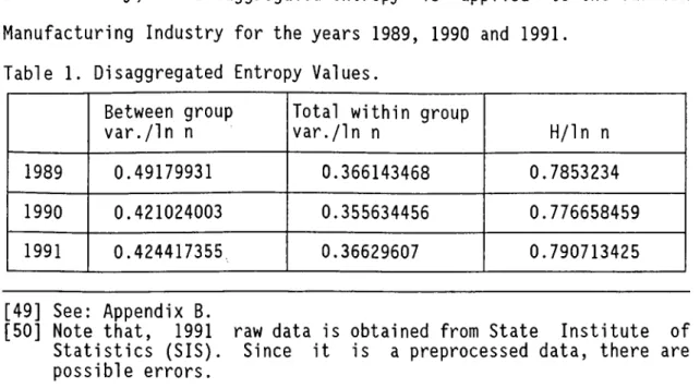
In this study, the disaggregated entropy is applied to the Turkish Manufacturing Industry for the years 1989, 1990 and 1991.
Table 1. Disaggregated Entropy Values. Between group
var./ln n
Total within group
var./ln n H/ln n
1989 0.49179931 0.366143468 0.7853234
1990 0.421024003 0.355634456 0.776658459
1991 0.424417355 0.36629607 0.790713425
[49] See: Appendix B.
[50] Note that, 1991 raw data is obtained from State Institute of Statistics (SIS). Since it is a preprocessed data, there are possible errors.
In the above table, to make the values independent from n, varying from year to year, the entropy values are divided by In n, thus the "relative" entropy values are considered in the computations, (where n is the total number of firms in the industry.)
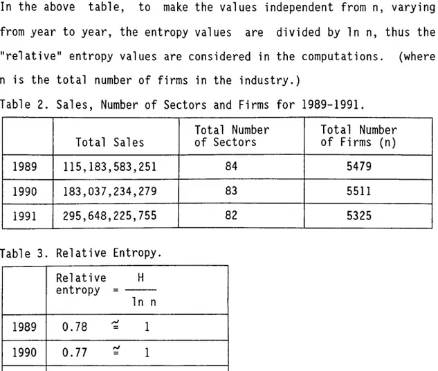
Table 2. Sales, Number of Sectors and Firms for 1989-1991.
Total Sales
Total Number
of Sectors Total Number of Firms (n)
1989 115,183,583,251 84 5479
1990 183,037,234,279 83 5511
1991 295,648,225,755 82 5325
Table 3. Relative Entropy.
Relative H entropy = In n 1989 0.78 = 1 1990 0.77 = 1 1991 0.79 = 1
It is obvious that there is a tendency to have equal shares in the industry. (There is not a tendency to a monopolistic situation. Level of concentration is very low (H— >1). The closeness of the values for the considered three years may point to some important facts about the Turkish Manufacturing Industry.
This study is conducted with the sales values. The computed 1989,
1990 and 1991 entropy values are very close to each other
emphasizing a certain continuity in the structure of the
manufacturing industry!
Yet, the main purpose of this study is to examine the intersectoral and sectoral changes rather than the general entropy values. Hence it
will be correct to compare the disaggregated entropy values. (Comparing the first and the second parts of the disaggregated formül a.)
One of the striking points for these three years is that - the between group variation values are higher than the total within group
variation values. What does this mean? The intersectoral
differentiation in the manufacturing industry are lower than the
within sectoral differentiation. Note that, the high levels of
differentiation seen in concentration analysis means getting closer to monopolization. As the differentiation decreases, the probability of having equal shares increases. For the three years considered, the sales distribution within the sectors displays a less equal pattern than the intersectoral analysis.
Let us compare the 1989, 1991 entropy values within the three years period. When the relative values are considered, the general entropy of 1989 is 0.7853234 while the 1991 value is 0.790713425.
As could be seen, the values are very close to each other. Here, it should be noted, the computed entropy indicates the deviation of the considered system's distribution from the homogeneous distribution. The general entropy index computed for the Turkish manufacturing industry, with the sales values, will not give the sectoral and intersectoral differentiations. Thus, the 1989 and 1991 entropy values above, which are close but still indicating a small (a very
small) differentiation, does not indicate the sectoral and
intersectoral situation for these years. (Still there is a slight variation between these two values.) Then the question arises: Is this variation due to one sector increasing its sales share as
opposed to other sectors or due to within sector sales share changes, or is it due to both factors simultaneously.
Note that, this analysis would give .a better result if this variation was more apparent. Although the values are close to each other and there is no apparent variation, the analysis can still be conducted.
When the 1989 and 1991 values are compared, the total-within group variations are almost equal. Thus, this means that the observed variation is due to the intersectoral differentiation rather than the within sector differentiations. The intersectoral entropy (between group variation) is equal to 0.41 in 1989 but attains the value of 0.42 in 1991. The intersectoral entropy increases but the total- within sector entropy remains constant. This two years' variation is due to one or few sectors' changing their shares within the whole manufacturing industry as opposed to other sectors, rather than changes of sales shares of firms within one sector.
According to the results of the calculation of Pb's, the sectors, whose shares had significant changes, are: 3114, 3219, 3232, 3319, 3543 3610, 3812, 3821 and 3829. The most important change is in the
two years' shard of 3319 and 3543. For 3319, the sale share
increased, from 0.000088 to 0.00027. For the sector 3543, the share is decreased, from 0.03578 to 0.00548. So, the slight difference between the general entropy values of 1989 and 1991 is due to these sector's changing their shares of sales within the manufacturing industry. Note that, this does not mean that the other sectors' shares are all remained the same during those two year period. But the changes will not effect the result, considering the changes in the number of firms in each sector during 1989-1991.
This analysis can be conducted for 1989-90 and 1990-91. For example, the change in entropy for 1989-90 period is due to both intersectoral entropy changes and the sum of within sector entropy changes. When the 1990-91 period is analyzed, the change in the value of the general (relative) entropy from 0.77 to 0.79 is due to some firms' changing the sales shares within one sector rather than intersectoral changes.
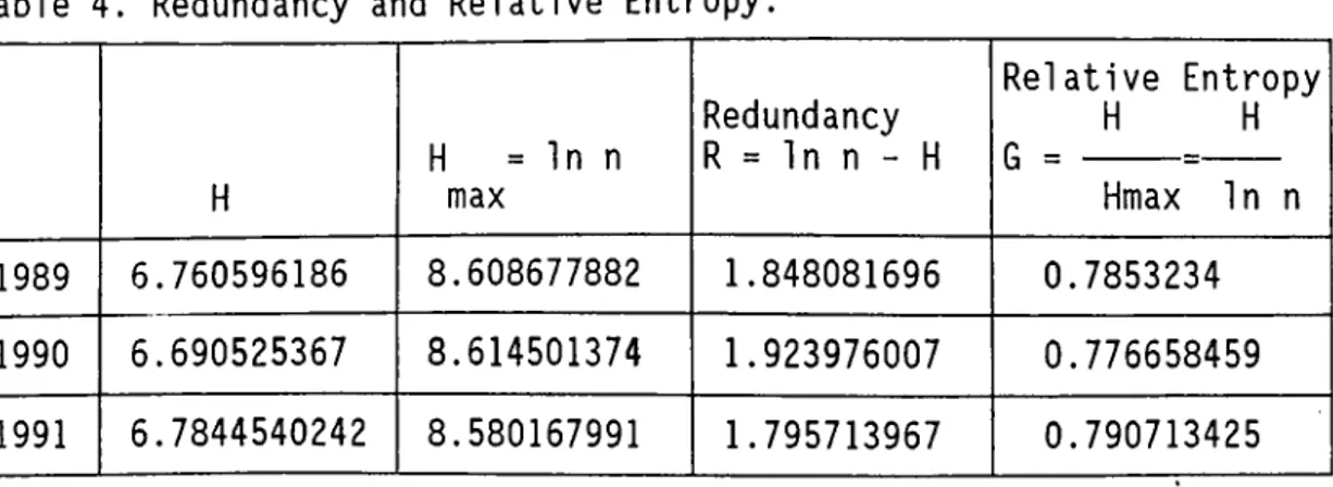
The maximum value of an entropy index is In n, where n is the total number of firms in the considered industry. When the maximum H values for 1989, 90 and 91 are compared, the entropy is closest to its maximum level in 1991. Thus, in 1991, the tendency of having equal shares of sales is the highest in the among the three years.
Table 4. Redundancy and Relative Entropy.
H H = In n max Redundancy R = In n - H Relative Entropy H H G = = Hmax 1n n 1989 6.760596186 8.608677882 1.848081696 0.7853234 1990 6.690525367 8.614501374 1.923976007 0.776658459 1991 6.7844540242 8.580167991 1.795713967 0.790713425
The decomposition of general entropy can also be interpreted just like as follows: "The degree of industry competition is measured as the weighted sum of the degree of competition in the individual markets plus the degree of competition that exists between the markets themselves" [51].
[51] Horowitz, I. (1971). Numbers-Equivalent in U.S. manufacturing industries: 1954, 1958 and 1963, Southern Economic Journal, Vol.37, pp.396.
"...one may use of 0 .^H<lnn, to obtain measures for the degree to which an industry is attaining its maximum possible dispersion of market shares or competitive potential, given the number of firms in the market" [52]. For this, Erlat states that we can either use redundancy [Hart, 1971 (pp.79)] or relative entropy [Horowitz, 1971 (pp.397)].
Redundancy = R Relative Entropy = G
= Iin 1-G)
(See: Erlat, 1975, pp.3é )
Inequality in the industry T» ^ ^ vt
Due to Erlat (1975), complete inequality = | R = In n complete equality
G = 0
= R = 0 = G = 1
1991 has the largest quantity of total sales between 3 years. The total sales figure for 1991 is 295,648,225,755. In this year, the largest share is that of petroleum rafineries, coded with 3530. The
petroleum rafineries have a share of 0.11 totalling to
34,828,983,348. The number of firms in this sector is 5.
In 1991, the sectors with the subgroup codes 3211, 3710 and 3843 follow the petroleum rafineries' sector.
Coming back to the petroleum rafineries (Sector 3530);
Table 5. Total Sales and Pb values for Petroleum Rafineries.
3530
Number of firms
in the sector Total Sales
Share in the manufacturing industry (Pb) 1989 5 13,310,232,785 0.1155566827 1990 5 23,058,688,845 0.1259781319 1991 5 34,828,983,348 0.1178054874 [52] Erlat, op.cit., pp.36.
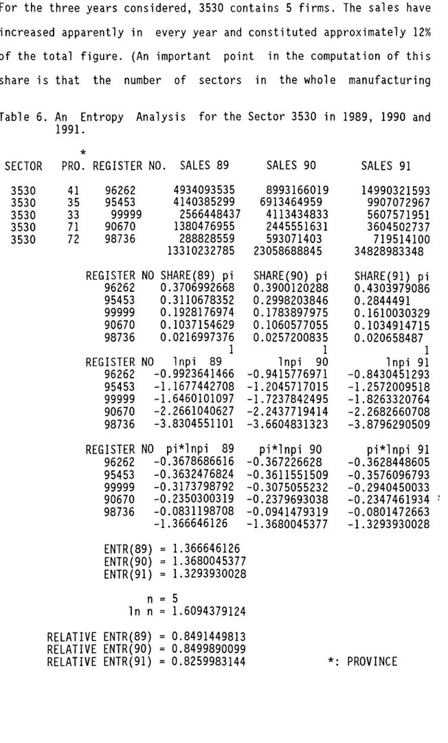
For the three years considered, 3530 contains 5 firms. The sales have increased apparently in every year and constituted approximately 12% of the total figure. (An important point in the computation of this share is that the number of sectors in the whole manufacturing
Table 6. An Entropy Analysis 1991.
for the Sector 3530 in 1989, 1990 and
SECTOR PRO. REGISTER N0. SALES 89
3530 41 96262 4934093535 3530 35 95453 4140385299 3530 33 99999 2566448437 3530 71 90670 1380476955 3530 72 98736 288828559 13310232785 REGISTER N0 SHARE(89) pi 96262 0.3706992668 95453 0.3110678352 99999 0.1928176974 90670 0.1037154629 98736 0.0216997376 1 REGISTER NO Inpi 89 96262 -0.9923641466 95453 -1.1677442708 99999 -1.6460101097 90670 -2.2661040627 98736 -3.8304551101 REGISTER N0 pi*lnpi 89 96262 -0.3678686616 95453 -0.3632476824 99999 -0.3173798792 90670 -0.2350300319 98736 -0.0831198708 -1.366646126 1.366646126 1.3680045377 1.3293930028 SALES 90 8993166019 6913464959 4113434833 2445551631 593071403 23058688845 SHARE(90) pi 0.3900120288 0.2998203846 0.1783897975 0.1060577055 0.0257200835 1 Inpi 90 -0.9415776971 -1.2045717015 -1.7237842495 -2.2437719414 -3.6604831323 pi*lnpi 90 -0.367226628 -0.3611551509 -0.3075055232 -0.2379693038 -0.0941479319 -1.3680045377 ENTR(89) ENTR(90) ENTR(91) n In n = 5 = 1.6094379124 SALES 91 14990321593 9907072967 5607571951 3604502737 719514100 34828983348 SHARE(91) pi 0.4303979086 0.2844491 0.1610030329 0.1034914715 0.020658487 1 Inpi 91 -0.8430451293 -1.2572009518 -1.8263320764 -2.2682660708 -3.8796290509 pi*lnpi 91 -0.3628448605 -0.3576096793 -0.2940450033 -0.2347461934 -0.0801472663 -1.3293930028 RELATIVE ENTR(89) = 0.8491449813 RELATIVE ENTR(90) = 0.8499890099
RELATIVE ENTR(91) = 0.8259983144 PROVINCE
industry is not the same in all 3 years. Because of this, the total sales figure does not include the same number of sectors in these 3 years. Thus, a possible comparison of a certain sector's share in the total sales figure may not be very healthy within three years.)
For the petroleum refineries sector (3530), this sector has the largest sales in the Turkish Manufacturing Industry, has increased its sales from 13,310,232,785 to 34,829,983,348 within the three year period from 1989 to 1991. A considerable increase was observed in sales.
The 5 firms in this sector (3530) are located in provinces coded 41,35,33,71 and 72.
As stated before 3530 with 5 firms, constitute approximately 12% of the total sales of the industry. But, how is the structure of this sector? Is the sales level of each firm constant and near to be equal or, in contrast, most of the sales is due to a single firm? Is there a tendency to monopolization? And, in addition, does this structure exhibit a significant variation within this three year period? This can be understood with an entropy analysis.
In the entropy analysis, the relative entropy of the sector 3530 are computed as; G(89)=0.8491, G(90)=0.8499 and G(91)=0.8259. As could be easily seen, the values are very close to maximum relative entropy value, 1, in all these three years.
As it is stated before, there is an important analogy between entropy and the competitiveness of an industry! Entropy's being closer to its maximum indicates the existence of a competition in contrast to monopolization. It can be said that the 5 firms' shares of sales are
close to each other and there is a very low concentration rate in the structure. This means that the sales share of 3530, which constitutes a major part of the total sales of the manufacturing industry is formed in a competitive structure.
It must be added that, the entry of new firms to this sector (3530) is not very easy. (As to the structure and characteristics of the sector.) This means that there will not be a frequent increase in the near following years. Thus, it will be highly unlikely that a possible variation will be caused by a change in n. (n can increase or decrease) There is a significant continuity in the structure of 3530, which has importance for the whole manufacturing industry.