Analysis of tip–sample interaction in tapping-mode atomic force
microscope using an electrical circuit simulator
O. Sahina) and A. Atalar
Electrical and Electronics Engineering Department, Bilkent University, Ankara 06533, Turkey
共Received 1 November 2000; accepted for publication 5 March 2001兲
We present a mechanical model for the atomic force microscope tip tapping on a sample. The model treats the tip as a forced oscillator and the sample as an elastic material with adhesive properties. It is possible to transform the model into an electrical circuit, which offers a way of simulating the problem with an electrical circuit simulator. Also, the model predicts the energy dissipation during the tip–sample interaction. We briefly discuss the model and give some simulation results to promote an understanding of energy dissipation in a tapping mode. © 2001 American Institute of
Physics. 关DOI: 10.1063/1.1369614兴
There have been many attempts to model the tapping-mode operation of atomic force microscope.1–7Some authors tried to solve the problem analytically2,6 and others at-tempted to solve it with computer simulations,3–5,7both add-ing to a better insight in understandadd-ing and treatadd-ing the data collected. It is now possible to map local energy dissipation profiles. We hope that a better modeling of the problem will lead to better imaging ability.
Early models neglected attractive forces and treated the tip as a forced oscillator hitting a damped elastic surface.2By using boundary conditions on the surface, the differential equation resulting from this model was solved. More in-volved models take attractive forces into account as well. This was hard to solve analytically, but numerical ap-proaches succeeded in explaining many experimentally ob-servable effects like attractive and repulsive regimes,4 hys-teresis in the frequency sweep,3 and bistability.5 However, these models did not take hysteresis in the adhesive forces into account, which was later shown by Tamayo and Garcia8 that this is the main source of energy dissipation in a tapping mode. Some recent works treat the interaction forces as a double valued function and solve the resulting differential equation numerically.7The results of this simulation showed the asymmetry of the necks formed by the sample surface during approach and retraction.
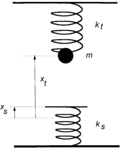
In this letter we present a model, which takes all the previously discussed effects as well as hysteresis. The model treats the tip as a forced oscillator, as usual. The sample is modeled with an equivalent spring constant1 共contact stiff-ness兲 and a damping effect, which is due to the internal vis-cosity of the sample. There is a negligible equivalent mass of the sample that we will totally neglect in this work. Interac-tion forces due to adhesion, surface charges, and some other sources are defined as a single valued function of the dis-tance between the tip and sample surface (xt– xs). The sche-matic of the model is sketched in Fig. 1. It is important to note that, although the interaction force is defined as a single valued function of the distance between tip and sample, the resulting force–distance relation exhibits hysteresis. Since
the attractive forces between tip and sample are proportional to 1/(xt– xs)n, there may be more than one stable solution5 for the sample position xs. When the tip approaches the sample, the level of the sample surface increases because of the attractive forces. After a certain point, the system be-comes unstable and the sample surface jumps to contact with the tip. However, during retraction, the contact is lost at a higher sample surface level. This results in different force– distance relations during approach and retraction.
In order to estimate the spring constant ksof the sample, we used the Hertz model applied to deformable bodies.1,2,7 When the model is applied to the tip–sample interaction, the equivalent spring constant is given by the formula
ks⫽32E*
冑
R⫻zdef . 共1兲 Here R is the effective radius of the tip, E* is the effective elastic modulus of the system, and zdefis the deformation of the sample. This value changes with force applied to the sample. Therefore, a nominal value of force is needed to estimate the spring constant of the sample. The best choice of this value is the adhesion force, since it is observed when no external force is applied to the tip and reflects theequi-a兲Electronic mail: [email protected]
FIG. 1. Mechanical model of the tip–sample system. Upper spring repre-sents the cantilever and the lower spring reprerepre-sents the sample. Damping of the cantilever and sample are not shown.
APPLIED PHYSICS LETTERS VOLUME 78, NUMBER 19 7 MAY 2001
2973
librium position.1Also, the forces observed in tapping modes are around this value. The equivalent spring constant can be written in terms of this force as
ks⫽
冑
36E*2RFadh. 共2兲
This parameter has a wide range, since elastic modulus var-ies by several orders of magnitude. The most important ap-proximation we have done up to now is to assume that this spring constant would be applicable also when the surface is pulled up. That is mainly because the forces of adhesion are effective at very short distances and, therefore, the surface is pulled up from a small volume in the vicinity of the tip. This is similar to the repulsion where the force is applied from a
small contact area but to the opposite direction. By making this assumption, we can then write the resulting coupled dif-ferential equations of motion as
md 2x t dt2 ⫹ m0 Q dxt
dt ⫹kt关xt⫺asp兴⫺F共xt⫺xs兲⫽A cos共t兲,
共3兲 ␥s
dxs
dt ⫹ksxs⫹F共xt⫺xz兲⫽0, 共4兲
where m, k, 0, , Q, asp, and A are the mass, spring con-stant, free resonance frequency, excitation frequency, quality factor, set point, and driving amplitude of the tip,
respec-FIG. 2. Equivalent electrical circuit of the mechanical model presented in Fig. 1. Left-hand side loop represents the cantilever–tip system and the right-hand side loop represents the sample. Diamond shaped symbols stand for voltage-controlled voltage sources. F(Vt⫺Vs) represents the force of interaction between tip and sample. Constant voltage source, V0is used to
adjust the set point.
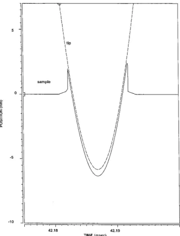
FIG. 3. Simulated tip–sample positions with respect to time. The solid line shows the position of the sample and the dashed line shows the position of the tip. The height difference of the sample right before and after the contact results in an energy dissipation.
FIG. 4. Simulated force–distance curve of the tip. Although the tip–sample interaction forces are defined single valued, the resulting force curve shows a hysteresis. The glitches are due to convergence problems and they de-crease with smaller time steps.
FIG. 5. Calculated energy dissipation with respect to contact stiffness ks.
tively, and␥sand ksare the internal damping coefficient and contact stiffness of the sample. xtand xs represent the posi-tions of the tip and sample surface, respectively, as measured from the equilibrium point of the sample.
Since we are dealing with masses and springs to model the problem, we can easily convert them to electrical circuit components. We replace masses with inductors, springs with capacitors, damping with resistors, and forces with voltages. The interaction force is represented by a nonlinear controlled source. The resulting electrical circuit is depicted in Fig. 2. We can then write the coupled differential equations for the charges qtand qs, of the capacitors as
Ld 2q t dt2 ⫹Rt dqt dt ⫹ qt Ct ⫺F共qt⫺qs兲⫽A cos共t兲⫹V0, 共5兲 Rs dqs dt ⫹ qs Cs ⫹F共qt⫺qz兲⫽0. 共6兲
The complete analogy between the mechanical and electrical system makes it possible to simulate the mechanical problem with an electrical circuit simulator such asSPICE.9This pro-gram can make a transient analysis of nonlinear circuits to predict the node voltages and branch currents. We preferred to useHSPICE,10a commercial version ofSPICE, which incor-porates very efficient algorithms for fast solution of nonlin-ear circuits. Since HSPICE does not allow charge controlled voltage sources, we added two extra nodes (Vt and Vs) whose voltages are numerically equal to the charges qt and
qsin capacitors (qt⫽CtVCt,qs⫽CsVCs). The multiplications are achieved by two voltage-controlled voltage sources gains of which are numerically equal to the respective capacitor values. We give the correspondence between the mechanical model parameters and the electrical circuit parameters in Table I.
HSPICE allows us to define nonlinear voltage-controlled voltage sources as piecewise linear functions. For the func-tion F(qt⫺qs), we use values similar to those measured by Tamayo and Garcia.8 We made transient analysis on this circuit for typical values of set point共60 nm兲, force constant
of tip 共10 N/m兲 and surface 共25 N/m兲, quality factor for the cantilever 共250兲 and center frequency 共15.9 kHz兲. For the sample viscosity, we have found that its value does not affect the results and therefore we have chosen something smaller than the damping of the cantilever. The extra factor of 1000 in Table I is there simply to scale the element values into an appropriate range as required byHSPICE.11In Fig. 3 we give the positions of tip and sample during interaction and in Fig. 4, the forces of interaction with respect to the position of the tip.
The neck formed during retraction is longer than the one formed during the approach. This is due to the hysteresis in the forces. After the tip is totally separated, the energy stored in the neck is completely lost. Since this energy is smaller than the energy gained right before contact, there is net dis-sipation. This dissipation is equal to the area inside the force–distance curve shown in Fig. 4. The value is approxi-mately a few hundred eV, which is similar to those experi-mentally measured values by Tamayo and Garcia.8In Fig. 5 we plotted the energy dissipation per tap with respect to the equivalent spring constant of the sample. These results show that energy dissipation in tip–sample interactions, which is a measurable quantity,8,12depends on elastic properties of the sample. Especially for compliant surfaces, energy dissipation can easily be related to local mechanical properties.
We have proposed a model to interpret the mechanism of energy dissipation in the tip–sample interaction in tapping mode. This will be useful in predicting energy dissipation profiles and mapping of local mechanical properties of samples. Furthermore, it is now possible to simulate the tap-ping mode operation much easier and faster with a circuit simulator.
The authors thank L. Degertekin of Georgia Institute of Technology and Mesut Meterelliyoz for helpful comments.
1
U. Rabe, K. Janser, and W. Arnold, Rev. Sci. Instrum. 67, 3281共1996兲.
2R. G. Winkler, J. P. Spatz, S. Sheiko, M. Moeller, P. Reineker, and O.
Marti, Phys. Rev. B 54, 8908共1996兲.
3A. Kuehle, A. H. Soerensen, and J. Bohr, J. Appl. Phys. 81, 6562共1997兲. 4
Ricardo Garcia and Alvaro San Paulo, Phys. Rev. B 60, 4961共1999兲.
5M. Marth, D. Maier, J. Honerkamp, R. Brandsch, and G. Bar, J. Appl.
Phys. 85, 7030共1999兲.
6L. Wang, Appl. Phys. Lett. 73, 3781共1998兲. 7
D. Sarid, J. P. Hunt, R. K. Workman, X. Yao, and C. A. Peterson, Appl. Phys. A: Mater. Sci. Process. 66, S283共1998兲.
8J. Tamayo and R. Garcia, Appl. Phys. Lett. 73, 2926共1998兲. 9L. W. Nagel,
SPICE2: A Computer Program to Simulate Semiconductor Circuits, University of California, Berkeley, Tech. Rep. Memo ERL-M520 共1975兲. A public domain version can be downloaded from www.repairfaq.org/ELE/F_Free_Spice.html
10
HSPICE: Avant! Corporation, 46871 Bayside Parkway, Fremont, CA 94538.
11
HSPICE, version 99.2 does not accept resistor values less than 10⍀. 12
J. P. Cleveland, B. Anczykowski, A. E. Schmid, and V. B. Elings, Appl. Phys. Lett. 72, 2613共1998兲.
TABLE I. Correspondence between the mechanical model parameters and electrical circuit parameters. The values given are the ones used in our simulations. Circuit parameter Mechanical equivalent Value Rt 1000 m0/Q 400 ⍀ L 1000 kt/0 2 1 H Ct 1/共1000 kt) 100 F Rs 1000␥s 100 ⍀ Cs 1/共1000 ks) 40 F F(qt⫺qs) 1000 F(xt⫺xs) ¯ V0 1000 ktasp 0.6 mV 2975