GROWTH, LIQUIDITY CONSTRAINTS, CREDIBILITY AND THE EFFECTS OF SHOCKS UNDER A NON-CREDIBLE GOVERNMENT

SHOCKS UNDER A NON-CREDIBLE GOVERNMENT Durmuş ÖZDEMİR(*)

ABSTRACT

This paper presents an overlapping generations model for a small open economy. The model is calibrated to fit data for Turkey. Simulations suggest that for a fairly open economy such as Turkey, credibility and liquidity constraints matter and the choice of income taxation rate, the mix of government spending and the long-run government debt/GDP ratio can all significantly affect the economic growth. The paper also examines the effectiveness of fiscal policy under different levels of liquidity constraint in an open economy within a dynamic framework. It shows that liquidity constraints can affect the outcome of any fiscal policy. Hence fiscal policy is even more important for the less developed economies of the world.

Keywords: Growth, liquidity constraints, credibility, the effects of shocks, fiscal

policy, calibration for Turkey.

1. Introduction

The objective of this study is to clarify the effects of the issues such as credibility, liquidity constraints and fiscal policy on the growth of the Turkish Economy. For this purpose, a popular approach to macroeconomic modelling, which is based on rigorous micro-foundations will be adopted. The advantages of the types of models used are ease of calibration which involves only a limited number of parameters associated with the utility of consumers and the production technology. As a form of forecasting, simulations generate a range of alternative projections based on differing assumptions about future situations. This approach concerns itself more with the question of ’what would happen If?’ rather than ’what will happen?’. Most simulation studies are carried out by altering the values of exogenous variables. Analysts can sometimes use particular simulation results to

derive standardised estimates of the consequences of economic policy action. Given the complexity of these types of simulation studies the use of computers has increased in importance. It is now a lot easier to do the rigorous calculations required with the aid of advanced packages and as consequence computer simulations have become increasingly popular amongst economists as a tool for analysing the behaviour of complex economic systems. Although complicated it is possible to perform controlled experiments with given economic systems. Simulation has made a substantial contribution to the testing of the effects of alternative government policies on the behaviour of a particular economic system. It is important for a macro-economic model to have a well-specified consumption function since this constitutes an important part of aggregate demand. In contrast to past consumption studies, which used constant variables, our simulation experiment will consist of dynamic variables exercised in a typical steady-state framework. It will attempt to describe the behaviour of a complex dynamic system, on a digital computer, over an extended period of time. The starting point of any computer simulation experiment is the development of a model of the system to be simulated. In the first part of this work it is proposed that a small open economy model of Turkey be developed. The model will be based on an overlapping generation framework Non-ricardian effects of government debt are important in this paper and occur for 4 reasons; Firstly, households leave no anticipated bequest for their heirs (Yaari, 1965 and Blanchard, 1985), secondly, debt neutrality breaks down due to existence of population growth (Weil, 1989), Thirdly, the government finances public expenditure on goods and services by distortionary taxation or borrowing (Yaari-Blanchard-Weil consumption function). Finally, the existence of liquidity constraints considered. A key feature of this model is its explicit recognition of both liquidity constrained and non-liquidity constrained consumers. Unconstrained consumers consist of overlapping generation, but apart from age, are identical. Turkish earnings distribution is very much skewed towards low income earners. As Vaidyanathan (1993) concluded 72% of Turkish people are liquidity constrained (unable to borrow) and only 28% of the population consists of unconstrained consumers. With this in mind it can be seen that the effect of any macroeconomic policy, in particular fiscal policy, would significantly different if the liquidity constrained consumers were not considered. The credibility of Turkish macroeconomic policy has long been on a considerably diminishing trend. Increasingly growing PSBR has trapped the state in a Ponzi-style financing of its debt. The inflow of short term capital may have been the only mode of adjustment

mechanism covering both the fiscal and trade deficit. A signal of a time inconsistency in the policy turned this inflow into a huge outflow which ultimately resulted in a severe recession. These developments raised the issues about the growth of the Turkish economy. The growth performance of Turkey’s economy in the last decade has been one of mini boom-and bust cycles. Turkey’s prospects for sustained growth have become more uncertain and chaotic. Hence issues regarding the effect of credibility of macroeconomic policies, liquidity constraints, and fiscal policy on economic growth have become even more crucial. Our model will be closest to that of Krichel, T. and Levine, P. (1996), which introduced liquidity constraints to a closed economy for India. In contrast to that of Krichel, T. and Levine, P. (1996) our model will consider an open, not closed, economy. The second part of this research will comprise policy simulation exercises undertaken with the aid of the ACES (Analysis and Control of Economic Systems) software. When examining a policy is important to compare the actual and desired paths of a target variable. Firstly the model is tested for stability. Long-term values of target variables and the trajectories of these variables are then observed. Hence, policy implications of the model are examined both theoretically and empirically. The simulation package ACES consists of three parts. The simple rule, the optimal rule and the time consistent rule, where each rules represents a different policy regime. For the Turkish case it would interesting to examine the time consistent and time inconsistent outcomes. Policies that are taken as optimal at one point in time may cease to be so later when optimization is recalculated, this policy may then become time inconsistent. This may have been the case in the previous anti-inflationary economic program. The policy then becomes sub-optimal. It has been argued that, in the absence of pre-commitment, the time inconsistent optimal policy is not credible (Currie, D. and Levine, P.1987). Therefore the time inconsistent policy only makes sense when a government has reputation for pre-commitment. Hence the credibility of the post-crisis economic policy is of major concern. The time consistent rule does not require reputation in this simulation. Policy rules such as the simple or optimal rules are of simple feedback form acting upon indicators, which provide information about the achievement of target objectives. Thus, a policy provides a simple mechanism through which it is to be revised in response to shocks, which offset the path of these variables from their desired course. Latterly

the simulation exercises will try to explain the effect of credibility, liquidity constraints and fiscal policy on economic growth.

2. The Model

A challenging model for this purpose has been developed by the following authors: Yaari (1965), Blanchard, O. (1985), Buiter, W. H. (1988) and Weil, P. (1985), Levine, P. and Pearlman, J. (1992), Levine, P. and Brociner, A. (1994), Krichel, T and Levine, P. (1995). Our model here will be closer to that of Krichel, T and Levine, P. (1995) which was taken as a closed economy example and applied to India. Here we will use similar setting but consider a small open, not closed, economy. Consumers are divided into two groups: constrained and unconstrained households. Unconstrained households behave as Yaari-Blanchard-Weil consumers and constrained households behave as Keynesian consumers. The consumption of constrained households is equal to their labour income but unconstrained consumers own all the financial and private physical wealth. Unconstrained consumers maximize an intertemporal utility function, subject to budget constraint. Firms also maximize an intertemporal profit function. The population growth and the labour supply is given. The domestic country’s consumer who born in period s has the following intertemporal expected utility function at time t ≥ s and there is no uncertainty apart from the probability of death. The aggregate utility function is

determined by (consumption of domestically produced good),

(consumption of imported good), (government provided domestic good),

(government provided imported good) and

s di C , s im C , Gdi,s s im G , t i

P

s

M

−

1

,

is the real money stock. All variables are at time i which is the beginning of the period.

∑

∞ = − ⎥⎦ ⎤ ⎢⎣ ⎡ + − = _{i t} t i s t p U

θ

1 1 , ⎥ ⎦ ⎤ ⎢ ⎣ ⎡ + + + + − t s i s im s di s im s di P M G G C C , 2 , 3 , 4 , 5 1,

1log α log α log α log α log

α

(2.1)

where denotes the price of domestic output, is nominal (high

powered) money stock and the θ is consumer’s pure rate of time preference.

t

Total consumption _{includes forgone expected interest payments on} money balances and is expressed with the following equation

) (Ct,s 1 , 1 1 , 1 1 1 , , ,

(

(

1

)

)

− − − − − −

−

+

+

=

t s t e t t t t nt s mt t s dt s t

P

M

t

t

R

C

E

C

C

π

_(2.2)

where

E

_t

=

real exchange rate

The expected asset return (taxed) is

R

_t

(

1

−

t

_t

)

where

t t t

Y

T

t

=

(tax ratio)

Assume real returns are taxed thus the effective expected nominal rate is

e t t t t nt

t

t

R

(

1

−

)

+

π

_+1, where

R

_nt is the nominal interest rate and

1 1 − −

−

=

t t t t

P

P

P

π

is the domestic inflation.

Consumption of domestically produced and imported goods is given byCdt,s =a1Ct,s, t s t s mt

E

C

a

C

_,

=

₂ , The demand for money is given by

e t t t t nt e t t t t

TR

TR

R

C

a

a

P

M

, 1 1 1 1 1 , 6 5 1 1

)

1

(

(

)

(

+ − − − − − −

+

−

+

=

π

The exante real interest rate

R

te

=

R

nt

−

π

te+1,t

This differs from the real interest rate which appears in the budget identities and refers to expost rate. Because of the credibility issue this distinction is important.

)

(

R

_t

s t s t s t t s t s t

D

F

K

P

M

W

, _{, , ,} ,

=

+

+

+

(2.3)

where is the government debt held by domestic or foreign consumers,

denotes net foreign assets denominated in home country and is the

domestic capital stock.

s t D_, s t F_, K_t,s

All assets measured at the end of the period. The consumer budget identity is given by

s t s t s t s t t s t T W w T C W_, = _{1 1,} + _, − _, − _, ∆ − − (2.4)

where ∆Xt = Xt −Xt−1,wt,s is the labor income, Tt,s denotes taxes

Maximizing (equation 2.1) subject to the consumer budget constraint corresponding to (2.4) provides Blanchard (1985) results.

s t

U ,

Expected aggregate consumption consists of the liquidity

constrained consumer’s consumption and the non-liquidity constrained consumer’s consumption.

)

(

e_1, t t

C

₊ rt t rt t t e t e t t R t nC p n p W w t nw C+_1, =(1+ (1− )−θ+ ) −( + )( +θ) −₁+λ(∆ (1− )−θ− ) (2.5)

Where λ is the proportion of the liquidity constraint consumers and n is the GDP growth ratio.

In (2.5), denotes rational expectations of formed at time t.

Assumed perfect foresight

e t t

C

_+1,

C

_t+1 1 , 1 + +

=

t e t t

C

C

The Government: The domestic country budget identity is given by

1 1 1

D

G

T

R

D

P

M

t t t t t t

₊

_∆

₌

₊

₋

∆

− − (2.6)

In terms of ratio ⎥ ⎦ ⎤ ⎢ ⎣ ⎡∇ + − + − + = _{− −} t t t t t t t t t Y P M n PDR DR n R DR (1 ₁ ) ₁ (

π

) _(2.7) where t t t

Y

D

DR

=

,

Y

P

M

MR

t t

t

=

and the primary deficit - GDP ratio is

is given by t

PDR

t t t t t t t

Y

T

Y

G

t

GR

PDR

=

−

=

−

The growth rate is

1 1 − − − = t t t t Y Y Y n

Solving the budget identity forward on time gives the solvency constraint:

∑

∞ = + + + + + + + + − + − + − + − = ₀ 1 2 1 1 1 ) 1 ...(( )... 1 )(( 1 ( i i t i t t t t t i t t _{R n R n R n} PD DR (2.8)

No ponzi game condition implies:

0 ) 1 ...(( )... 1 )(( 1 ( lim 1 2 1 1 1 ₌ − + − + − + _{+ + +}++ _{+ ++} ∞ → i t i t t t t t i t i n R n R n R PD (2.9) Assume no dynamic inefficiency

The debt accumulation:

t t t e t t t t t t R n m DR G T DR₊₁ =(1+ − ₋₁)[1− (

π

−

π

)] + −

(2.10) where = e t

π

the rational expectations of inflation

=

t

m

proportion of inflation sensitive debt (i.e. nominal long-term debt in domestic currency)

t t t t

R

F

TB

F

=

+

∆

_{−1 −1} (2.11) where TB_t =C_mt* −E_tC_mt +I_mt* −E_tI_mt +G_mt* −E_tG_mt = * mt

I Foreign investment out of domestic output.

=

mt

I

Investment out of imported goods

Starred variables such as * refer to the foreign.

mt C In ratio form: t t t t t

FR

TBR

n

R

FR

_⎥

+

⎦

⎤

⎢

⎣

⎡

+

+

=

− ₋ 1 1

1

1

(2.12) where t t t Y F FR = and t t t Y YB TBR =

Output, private sector and Investment It is assumed that the aggregate output is given by the following Cobb-Douglass production function:

2 1 2 1 1 1 1

(

)

β β β β − − − −

=

_{dt mt t t} t

K

K

A

L

Y

(2.13) = − 1 1 β dt

K End of period capital stock accumulated out of domestic output = − 2 1 β mt

K capital stock accumulated out of foreign output.

=

t

L

Exogenous labour supply

t t A

A = 0(1+

µ

) _{represents Harrod -neutral technical change where µ is the} productivity growth.

2 1

β

β

β

=

+

is capitals share of output. Steady state GDP growth =

n

=

µ

+

g

∑

∞ =0 + + i

l

t i

π

t i _(2.14) 1 1) 1 ( 1 − + − + + = _{t i} i t R l l ,

i

≥

1

;

l

t

=

1

Single period firms real income is:

mt dt dt t rt t t

=

Y

−

w

L

−

I

−

E

I

π

(2.15) where

w

_rt

=

real wage

Gross investment out of domestic and foreign output,

I

_dt and

I

_mt:

dt dt dt

K

I

K

=

(

1

−

δ

)

₋₁

+

mt mt mt

K

I

K

=

(

1

−

δ

)

₋₁

+

where

_δ

₌

depreciation rate

Total capital stock is

K

t

=

K

dt

+

E

t

K

mt

Firm takes the and real exchange rate over the planning period

exogenously.

t t

t w L

R, ,

The equilibrium in the output market gives:

t mt t dt mt t dt mt t dt t

C

E

C

I

E

I

G

E

G

TB

Y

=

+

+

+

+

+

+

(2.16) Firms equate the net marginal product of capital to the marginal cost of capital. From the first order conditions derived from the production function:

δ

β

+ = − − e t t dt R Y K 1 1 1 _and ) 1 ( ) 1 ( ₁ 1 2 1

δ

β

− − − − te te t t R E (2.17) where denotes the expected relative price.

+ = − mt E Y K e t E

3. Liquidity Constraints, Fiscal Policy and Growth in Steady State

From the equation (2.5), the steady state form of the Yaari-Blanchard consumption function is as follows:

) ) ) 1 ( ( ) )( )( ( ) ) 1 ( ((R −t −θ+nC== p+n p+θ K+D+F −λ R −t −θ+n w _(3.1)

The steady state values will be denoted without a subscript t. The elimination of C, K and G gives the following function which determines them in terms of R, n, D, t, γ and λ: 0 ) ) ( )( )( ( ) 1 )( 1 ( ) ( ) 1 ( ) ( ) ( ) ) 1 ( ( ) , , , , ( = + + + − − − − − − − + + − − = D R K p n p t R K t D n R R K n t R D R n f

θ

α

λ

δ

θ

λ

γ

(3.2) Where _C=(1−(n+

_δ

_)K(R)−

_λα

_(1−t) ) ) (r n D T G= − − ) (R K R K = + =

δ

α

The equation (3.2) is upward sloping and describes the locus of interest and growth rates consistent with Yaari-Blanchard consumption behaviour, output equilibrium, private sector investment and the government budget constraint.

A similar solution of the production function of the equation (2.13) gives: 0 )) log( ) ) ( ) ( 1 ( log( log )(log 1 ( ) ( log ) , , , , ( _{2 2} = + − − − − + + − + =

δ

δ

γ

γ

γ

γ

n D n R R K t A R K t D R n g (3.3) The downward sloping equation (3.3) is the locus consistent with balanced growth and private sector investment, the government budget constraint and the production technology.

Then examining the effect of capital stock on the interest rate in the steady state we begin by using the consumption equation for Yaari-Blanchard consumers in the steady-state. Solving equation (3.1) for R gives;

w

t

t

C

w

n

F

D

K

n

p

p

C

n

R

)

1

(

)

1

(

)

(

)

)(

)(

(

)

(

+

−

−

−

+

+

+

+

+

+

−

−

=

λ

θ

λ

θ

θ

_(3.4)

This is the function for the household’s supply of capital. We will now examine the effect of capital stock and liquidity constraints on interest rate with the aid of this function.

A simple way of conducting a comparative analysis would have been merely to calculate the sign of the derivatives of the steady state values of the interest rate with respect to K and λ. A positive sign for the derivative would indicate that the variable under inspection varies directly with K and λ, while a negative sign would indicate an inverse relationship. The precise effect of capital stock change on interest rate can be shown by differentiating R with respect to K which gives; 0 ) ( + _{(1 )((1 ( ) ( ) (1 )) (1 )} > = _{− − +} +_{− − + +} w t t R K n t n p p dK dR λ λα δ

θ

(3.5)

Wealth consists of the capital stock K, (for simplicity the total capital stock K=K+F+D).

Since Y’(K)=R and RK<Y(K), dR/dK>0, as required. The effect is positive and r varies directly with change on K in a positive way. In a completely liquidity constrained economy where lambda converges to one, then dR/dK is converging to zero. The reason for this is that as lambda converges to one consumption is equal to wages so that while the interest rate approaches infinity, the capital stock approaches zero. Because there are no savings there is no capital.

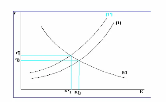
Figure 1:The household supply and demand

Taking the production function given in the equation (3.2) and solving for R satisfy the following condition and the demand for capital by firms is given by;

) (K

f

r = ;

_f

''

(

_K

)

_<

0

(3.6)

The household supply and demand for capital by firms are shown in Figure (1) which indicates the macroeconomic equilibrium where r* and K* are as

in the

figure. The next step is to examine the effect of a change in λ on the equilibrium. The effect of a change in lambda on ”R” can similarly be examined by differentiating ”R” with respect to lambda as follows,

0

2 ) ) 1 ( ) 1 ( ) ( ) ( 1 ((( )) 1 ( ( ) ( ) ) ((( ( ) 2 2 ))( 1 ( ) ( ) ( 1 ((

_>

−

=

− + − ₋−₊ − ₋+ _{− +}+ ₊+ + + + + w t t R K n t n n t n p p K t n t R K n d dR

_w

λ λα δ θ θ θ θ λα δ λ (3.7)

The effect is positive and R varies directly with changes in λ in a positive way. Since (K)>Rk curve (1) in Figure (1) shifts left as λ shifts. This Figure shows the affect of lambda increasing on the steady state capital stock and interest rate.

The household’s supply of capital function, curve (1) in figure (1) is derived from equation (3.4). The demand for capital by firms is given by curve (2) in figures (1) which is derived from equation (3.6). A higher lambda leads to a higher ”R*” and lower ”K*”. The reason for this is that liquidity constrained households do not accumulate capital. ’K*’ and ’R*’ gives the macroeconomic equilibrium. In the limit as lambda approaches one, C approaches “w”, K approaches zero.

3.1 Ricardian Equivalence, Liquidity Constraint and Fiscal Policy.

Barro (1974) argued that fiscal effects involving changes in the relative amount of tax and debt finance, for a given amount of public expenditure, would have no effect on aggregate demand, interest rates and capital formation. In this section our aim is not only to consider whether Ricardian equivalence fails or not but also to consider all alternative options within our model. We will now examine the Ricardian equivalence discussion in terms of the equation (3.4). The cases we are going to discuss are: Ricardian, Ricardian no-liquidity constraint, non-Ricardian with liquidity constraint and non-non-Ricardian where all consumers are liquidity constrained. The Ricardian case in our model means that the probability of death is equal to zero. This is the case where all individuals are concerned about future generations. Our model’s flexibility clearly shows that it is possible to examine all possible cases within the model framework.

Ricardian; If Ricardian equivalence is valid, then the case would be

represented as p=0 in our model, i.e. p is the probability of death which is zero in the Ricardian case. Solving equation (3.4) under this condition provides us

w t t C w n K n C n R ( ) ₍(₁₎)( ₍₁) ₎( ) + − − − + + − − = θ θ _λ λθ

Non-Ricardian, no liquidity constraints; This is the case where probability

of death is greater than zero but there is no liquidity constraint, λ=0. This is the case in the original Yaari-Blanchard model. Interest rate greater than θ , (when p>0, λ=0 and r>θ), and individuals have shorter horizons hence “R” becomes;

K p n p

n

R

₌

_θ

₋

₋

( + )( +θ)

According to this outcome Ricardian equivalence might fail even though there are no liquidity constrained consumers present. We will be examining the case, in more precise terms in a later section, of how non-Ricardian the Yaari-Blanchard model is.

Non-Ricardian, liquidity constraints; According to empirical investigations

this is one of the most likely cases in our model because, as we have argued, the probability of death is greater than zero and some proportion of aggregate consumers are liquidity constrained. This can be presented as p >0 and 0 <λ <1. In this case R is likely to be larger than the R for the case of non-Ricardian, no liquidity constraint. w C K p n p

n

R

=

θ

−

−

( + )(_−λ+θ)

A change in capital stock affects interest rates and consumption at the steady state level, this change depends on the proportion of lambda. Any changes in interest rates caused by capital stock will be different under conditions of various liquidity constraints. These results clearly show that the Ricardian equivalence proposition would be affected by the proportion of liquidity constrained consumers in an aggregate consumption function.

Non-Ricardian, all consumers are liquidity constrained; This is where all

consumers consume their current income, λ=1, p>0, being an extreme case. There is no capital, K and hence no interest rate; consumption is equal to the post tax labour income w. This implies no Ricardian effect.

How non-Ricardian is the Yaari-Blanchard consumption function;

The analysis is extended to examine how Ricardian or non-Ricardian the Yaari-Blanchard model is. After introduction of debt, D, government expenditures, G, and the Foreign asset,F, to our model then equation (3.4) would be in the following form: w t R K n F D K p n p n R=

θ

− −₍₍₁₋(_{( +}+_δ)(_{) (}+θ₎)(_−λα+₍₁₋+₎₎)_−λ

where debt is part of wealth. In terms of labour income ratios, the last equation would be in the following form:

w t R K n FR DR KR p n p n R=

θ

− − ₍₍₁(₋₍+₊)(_δ)+θ₍)(_)−λα+₍₁₋+_))−λ)

where ∆DR=(1+R−n)DR+PDR

These are shown in terms of ratio where

_DR

₌

_YD_{, the primary deficit -}

GDP ratio is PDR, given by Y T Y G

TR

DR

PDR

=

−

=

−

and

KR

=

K

/

Y

,

This last equation simply states that the interest rate is affected by these ratios and the last equation is derived from the Yaari-Blanchard consumers’ consumption function.

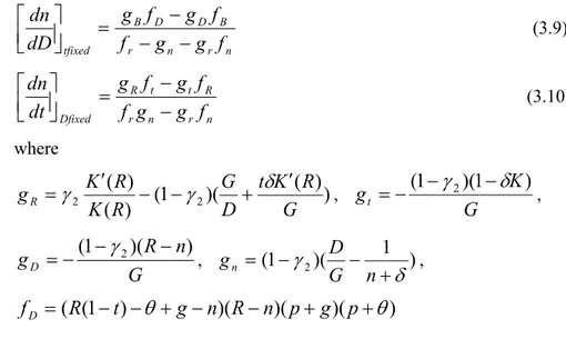
If λ shifts then the supply of capital (1) curve shifts upwards too because savings are lower and the capital stock is smaller compared to the case with no liquidity constraints. Figure (2) indicates that in an open economy an increase on G/Y or D/Y shifts the household supply curve from (1) to (1’). Hence an increase in a case where lambda is greater than zero means that GR and DR

would shift the supply curve towards the left and this shift would give a higher level of interest rate.

3.2 Debt Capital Stock and Liquidity Constraints

We shall now examine the effect of the level of government debt on capital stock in the steady state. For this examination we will assume government expenditures are fixed. D denotes debt as a part of wealth and enters the consumption function and the interest rate is replaced by the marginal product of capital, Y’(K)-δ. We have differentiated K* wrt. D* after substituting these definitions in to equation 3.8 so that in steady state the following result is achieved;

w t t R K n t n p dD dK _p ) 1 ( )) 1 ( ) ( ) ( 1 )(( 1 ( ) ( + _{− − +} +_{− − + +} =

θ

_{δ λα λ} for p>0 and λ<1. (3.8)

If lambda is equal to zero then an increase in D* has the same effect on the steady state capital stock as in the Yaari-Blanchard Model. This examination is carried out when G is constant. Equation (3.8) could be positive or negative depending upon the values of its parameters. Parameters p, q, λ, C, Y and (D+K)

and the denominator could be positive with a reasonable values of the parameters. If the derivation of the equation is positive then, for instance, an increase in debts would increase the steady state capital stock. If dK*/dD* is negative then we have an important result; for example an increase in debt decreases the steady state level of capital stock. Suppose the government cuts taxes, holding its spending constant. This would raise the deficit and increase the debt. If an increase in the steady state level of debt decreases the capital stock then we have an inefficient outcome. It is inefficient because an increase in borrowing decreases output and hence consumption. A reverse policy, i.e. a decrease in debts to increase consumption, could not be an option because (due to previous tax increase) this would increase the budget deficit further. If interest rates increased to a positive level then an increase in debts could increase the steady state capital stock and hence consumption.

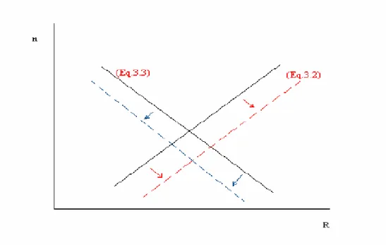
Figure 2 indicates an effect of increase on G/Y and D/Y to household supply curve, which shift unambiguously.

3.3 Long-run Growth

The derivation of multipliers from the equation (3.1) provide the effect of debt/GDP and the tax/GDP on long-run economic growth.

n r n r B D D B tfixed

f

g

g

f

f

g

f

g

dD

dn

−

−

−

=

⎥⎦

⎤

⎢⎣

⎡

(3.9) n r n r R t t R Dfixed

f

g

g

f

f

g

f

g

dt

dn

−

−

=

⎥⎦

⎤

⎢⎣

⎡

_(3.10) where

)

)

(

)(

1

(

)

(

)

(

2 2

G

R

K

t

D

G

R

K

R

K

g

_R

=

γ

′

−

−

γ

+

δ

′

,

G

K

g

_t

₌

₋

(

1

−

γ

2

)(

1

−

δ

)

_,

G

n

R

g

_D

₌

₋

(

1

−

γ

2

)(

−

)

_{, (1 )(} 1 ₎ 2

_δ

γ

+ − − = n G D gn ,

)

)(

)(

)(

)

1

(

(

−

−

θ

+

−

−

+

+

θ

=

R

t

g

n

R

n

p

g

p

f

_D

))

1

(

1

)(

)

1

(

(

−

−

θ

+

−

−

δ

+

λ

−

α

−

−

=

RC

R

t

g

n

K

f

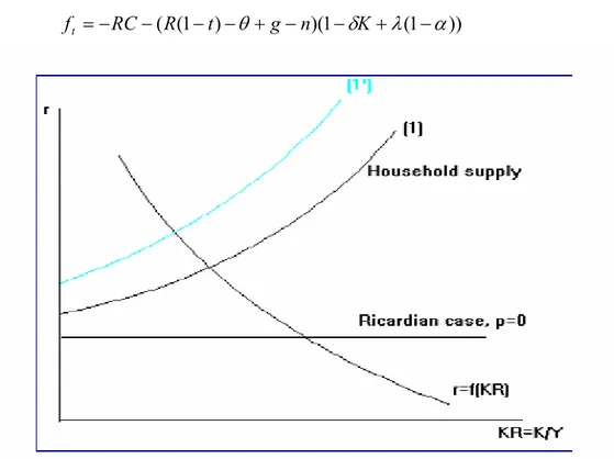
_t

Figure 2: The effect of increase on G/Y and D/Y to household supply curve, shift up unambiguisly

Figure 3: The effect of D/Y change on growth ) ( ' ) )( ( ) 1 ( )) ( ' )) 1 ( ( )( ) 1 ( (R t g n D n t K R C t p g p K R fR= − −θ+ − − +δ − + − − + +θ ) )( ) 1 ( (R t g n K D C fn =− − − −θ+ − +

Keeping fiscal policy fixed, the effect of R on growth from the derivation of the (3.1)

( )

_∂∂_Rn _{f=0 has a positive sign: as R increases the steady state growth}

increases too. Indicates an upward slope between the steady state growth and the rate of interest in Yaari Blanchard consumers.

Keeping fiscal policy fixed the effect of interest rates on growth from the derivation of the (3.2)

( )

_∂∂_Rn _{g=0 provides a negative sign as R decreases n increases.}

The effect of an increase in debt (D) on the steady state growth (n), where t and γ are fixed is negative. That is

( )

_∂∂ _,

<

0

fixed t

Dn γ . This result has interesting

suggestions: Steady state growth can be increased by reducing the debt/GDP ratio. Figure 3 indicates the effect of D/Y change on growth. Curve (3.2) shifts right (R and t fixed) as a result of increase on debt/GDP ratio. Similarly keeping R, t and γ fixed in the equation (3.3): an increase of D/Y on growth shifts the equation (3.3) left. Hence an increase on debt/GDP ration decrease the long run growth but has an unambiguous effect on R.

For example an increase in tax ratio (when D/Y and the production technology are constant) on long run growth in this model is ambiguous too. That is

( )

∂_{∂ ,}

=

?

fixed D t n

γ . Hence we will leave this effect for calibration.

Calibrations of these multipliers for the Turkish economy are present in the simulation results section. For a further details of the models’ derived multipliers see Levine and Krichel (1995).

4. The Model Simulation

In this part we will be altering some parameters of the model and will assess the likely impacts of various fiscal policies. Firstly, we will calibrate the model and the simulation of this model using different liquidity constraint levels of an economy will be carried out. This simulation will be providing further evidence for the implications of liquidity constraints on fiscal policy. The optimal program, which is reputational calculates the optimal policy. The program presumes that the private sector will believe implicitly whatever policy announcement the government makes. Non-reputational TCT program calculates best time consistent policy. Under these two programs, simulation of optimal growth will be carried out. The effect of the different levels of D/GDP and λ values on growth will be scrutinized.

Maximizing the social utility is equivalent to minimizing the quadratic welfare loss. In our study the below welfare loss is generalised into the following form so that it would include the tax distortions. Thus the welfare loss function

2 6 2 5 2 4 2 1 3 2 2 2 0 1 1

)

(

)

(

)

(

)

(

)

(

)

(

(

1

1

π

π

α

α

α

α

α

α

θ

−

+

−

+

−

+

−

+

−

+

−

⎟

⎠

⎞

⎜

⎝

⎛

+

−

=

+ + + + + ∞ = +

∑

i t i t i t i i t i t i t

m

m

d

d

t

t

g

g

c

c

p

W

(4.1)

Where t is taxes, c is consumption, g is government expenditures, m is real money balances, d is debts in terms of ratios and π is the rate of inflation. The fourth term in this equation is necessary to ensure government solvency in the strong sense that the debt/GDP ratio must be stable. The third term captures the distortionary effect of taxation.

The optimisation process in the ACES minimises a welfare loss, which must be in the quadratic form, and maximises the social utility is equivalent to minimizing the welfare loss.

The simulation of this model is carried out by using a linear software, ACES. Linear solutions are used in the non-linear model to provide either approximately consistent solutions, or to assist in the specification of the terminal conditions for the expectational variables required in the non-linear procedures. Thus this model is firstly linearized in the region of the steady-state which we have already found. The linearization is done by using the Taylor series approximation. It is also convenient to express C,Wand w as proportional derivations. For example, for C, _c= C_C−C _{, and for}

W W W

w₌ −

We will be treating some of these parameters as the fundamental parameters and some of the others as the derived parameters.

4.1 The Summary of Calibration.

Our calibration strategy begins by calibrating the steady state values of selected variables. These variables are presented below in the summary of calibration such that the government expenditure, capital stock and debts are taken as the ratios of output. The deep parameter values such as θ are chosen by calibrating the steady state values of selected parameters. There are a number of studies which have estimated consumption functions with liquidity constraints. We have taken 0.72 for the proportion of liquidity constrained consumers from the Turkish example. This estimate, as we have discussed differs for different economies and is rather higher for LDC’s therefore we will examine some different

levels of λ in our simulation analysis. Some of our fundamental parameters’ steady state values are taken from State Institute of Statistics (SIS) data source of Turkey. Our microeconomic foundation model in which consumer maximize utility and producers maximise profits, is consistent with observed data. The rates of return, i.e. R+δ, is equal to 0.17 which is the real interest rate plus the depreciation rate. The average probability of death per year is taken as 1/40, as it is consistent with Turkish life expectancy. The OECD figure for K/GDP average is taken as 2.5. The rest of the parameters and sources are presented in the summary of calibration as follows. The model parameters are divided into two groups; fundamental parameters and the derived parameters. These are as follows:

Fundamental parameters and their source:

1. Marg. prod. Capital, R + δ = 0.17 Turkish average reel rates of interest for 1990-2000, SIS.

2. p= 1/life-expectancy for working age = 1/40 (Average life expectancy of last 3 decades in Turkey, SIS)

3. δ = 0.07 (Average of 1990-2000, SIS, Turkey) 4. β = 0.3 OECD

5. λ =0.72 (Vaidyanathan, G. (1993)Turkey)

6. G/Y = =0.2 (Average of 1990-2000, SIS, Turkey) 7. K/Y = 2.5 OECD

8. D/Y =0.6 (Average of 1990-2000) SIS, Turkey) 9. π = 2 ( Average population growth, 1965-2000, SIS) 10. n =4 ( GDP growth, 1990-2001, SIS

11. DIS 0.95 (Myopic government, assumed)

Derived parameters

12. C/Y = 1− G/Y = 0.8 13. T/Y = RD/Y+ G/Y = 0.26

14. 15. W/C = 4.429 16. w/C = 0.921 17. C(YB)/C = 0.816 18. w/Y= 0.645 19. K/W = 0.806 20. D/W= 0.194

21. ((1−p)/(1+θ)) = 0.908(Government discount rate). 22. ˆC = 100 23. ˆg = 100 24.ˆt = −23 25. ˆd= −60 26. α1 = 1 27.α2 = (G/Y)/(C/Y)= 025 28. α3 = 0.1 29. α4 =0.1

If DIS = 1, in the equation, then the government in effect chooses the same discount factor as the private sector. If DIS <1 , then the government is more myopic. These are the steady state values of our model parameters. We will be examining the deviations of these values.

4.2 Simulation Results.

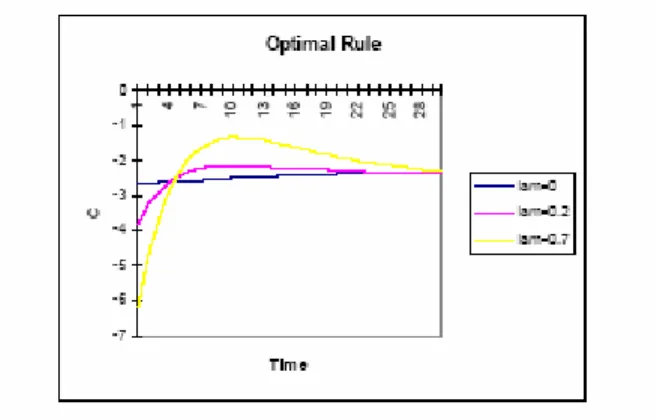
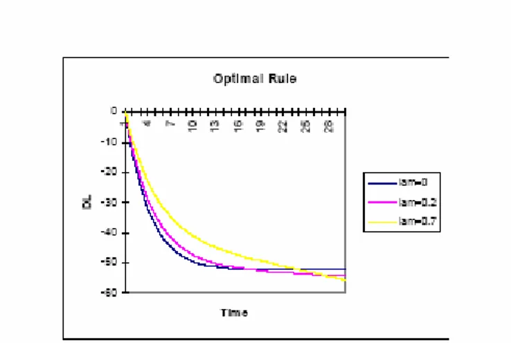
Two types of policy rules are provided by the package: the optimal rule requires reputation for precommitment and the dynamic programming time consistent rule which does not require reputation. The outcome of the model under these rules is examined. Firstly we tested the stability of our model with rational expectations. The program computed the eigenvalues of the system and reported that saddlepath property holds. When saddle path property held then the program computed the trajectories of all the model variables for the required 30 years time

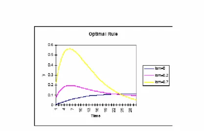
period. Figures 1 - 8 present these trajectories of D/Y, C/Y and y under different levels of liquidity constraints with two policy rules. A number of features of these results are worthy of comment. With consideration of the two policies, i.e. TCT and OPTIMAL, under four different levels of liquidity constraints, i.e. 0 and 0.7, no matter which policy is implemented, different liquidity constraints create different trajectories for the selected variables, i.e. C, D/Y and y. The greater the liquidity constraints, the bigger the deviation from the baseline steady-sate values of these parameters. The highest deviation from steady-state values can be seen in the figure for y. These trajectories clearly show that liquidity constraints matter. In the final stage we imposed some parameter changes, i.e. variations of lambda and a change on tax ratios.

We also examined the results under permanent or temporary shocks. The trajectories are always given in terms of displacements from the initial equilibrium. When shocks were permanent then the program calculated the new equilibrium values and also provided the new welfare losses for a particular time period. In the case of OPTIMAL the private sector believes the government’s announced policy. The program works by minimising the welfare loss function, which we presented in equation 4.1. An examination of the trajectories in figures (1) - (8) highlighted that the two different policy regimes; TCT and OPTIMAL, are very similar under different levels of liquidity constraints. However, higher is the level of liquidity constraint consumers, bigger is the fluctuations in output after shocks. Hence a higher λ means that the supply shocks cause more instability and bigger fluctuations compared to the lower levels of liquidity constraints. The higher the lambda values, the bigger the fluctuations. As a result, a higher proportion of liquidity constrained consumers brings more instability because, as we argued previously, the reaction of these consumers to any shocks would be greater compared to non-liquidity constrained consumers. Higher liquidity constrained consumers imply lower capital stock and the effect on interest rate is smaller. If lambda is greater, TCT and OPTIMAL outcomes differ greatly. This indicates that the reputational policy is even more important for a country such as Turkey. However, if, for example, λ = 0, TCT and OPTIMAL results are very close. This is because, as was argued in Levine and Holly (1987), time inconsistency arises from the private sector. The

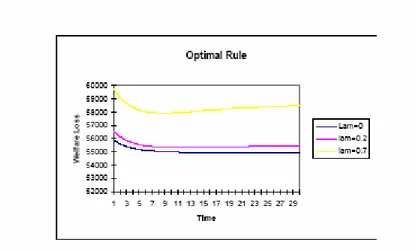
Yaari-inconsistency due to the behaviour of private agents. The behaviour of forward looking agents however is more certain as was the case in the original model. The TCT program uses the dynamic programming solution assuming that government has no reputation and simulates a particular policy over time. In all programs trajectories are given for all variables and long run values only calculated when shocks are permanent. We have firstly run the model with original specification, i.e. with the calibrated parameters in the calibration summary; the λ value is equal to 0.72 for two policy regimes. The variables are in percentages and measured as deviations about the original steady-state. For example where R = 0.10 in the calibration. The first simulation is about the levels of various liquidity constraints under different policy rules. The second is a fiscal policy exercise in which there is a 10 percent increase in government debts (an increase in D/Y). This increase is also examined in the case of different liquidity constraints. Finally, in order to examine the temporary and permanent fiscal shocks under various levels of liquidity constraint a temporary shock is introduced to the system. Figures show the effect of the liquidity constraints. We examined the range of liquidity constraints by altering the initial value of λ = 0.72 for two policy regimes, i.e. optimal, and TCT. A higher proportion of liquidity constrained consumers in an economy causes higher welfare losses and this result does not change under the two different policy rules. Under the optimal control, reputational and time consistent rules; higher lambda requires a higher steady state level of taxes and higher capital/GNP ratios.

The differing proportions of liquidity constrained consumers also affects interest rates ( R ) and the output (y ). If an economy has a higher level of interest rates then this gives a higher proportion of liquidity constrained consumers and a lower output level because higher interest rate leads to a lower investment hence lower output. An important point is that when the liquidity constraint is higher, such as 0.7, as in the case of optimal control rule with reputation, the Yaari-Blanchard consumer’s consumption is not decreased as much as the decrease on the liquidity constrained consumers, under the imposed tax increase. When a policy authority imposes a higher tax ratio, the effect of this fiscal change very much depends on the proportion of liquidity constrained consumers. Most of the decrease in consumption goes to the liquidity constrained consumer’s consumption. However, it is possible to argue that the specification of tax, i.e. instead of income tax, a VAT, may change the result further, against the liquidity constrained consumers. A similar effect can be observed in the time consistent regime. If the proportion of liquidity constrained consumers is higher, such as 0.7 (this is the case for most developing countries and Turkey) then fiscal policy is more effective. This result clearly indicates that fiscal policy is more important for underdeveloped countries than for developed countries with developed consumer credit markets. The proportion of lambda makes a difference for the outcome of a fiscal policy.

Figure 6: Effect of shock on D/Y under time consistent rule

Figure 10: Effect of shock on welfare loss under time consistent rule

One long standing argument is that if an economy consists mostly of permanent income consumers, in this case the Yaari-Blanchard consumers, then temporary shocks should not affect the level of aggregate consumption to a great extent. In the case of higher liquidity constrained consumers, the temporary shocks may provide less welfare losses. By comparing the previous tables there is a significant difference between temporary and permanent shocks for the welfare loss criteria. Fiscal policy certainly affects aggregate consumption regardless of the shocks, whether temporary or permanent, which contradicts Barro’s (1974) argument because probability of death is not zero and some consumers are liquidity constrained. It may be concluded that in an economy, such as a developing country’s economy, temporary fiscal shocks can provide smaller welfare losses compared to the economies which have less liquidity constrained consumers. These results coincide with a long standing argument that temporary shocks, in a highly liquidity constrained economy, can provide less welfare loss compared to the permanent shocks while these shocks may not be very effective in the economies which have a lower proportion of liquidity constrained consumers. This proportion, λ, clearly affects the outcome of any fiscal policy. As we argued, fiscal policy even more important for an economy which has a high proportion of liquidity constrained consumers. Furthermore, as ultimate objective, the effect of government expenditure, taxes and in particular government debt on long-run growth is a prime concern for the Turkish economy.

4.3 Optimal Growth, Calibration and Numerical Results for Turkey

The key question is that the effect of Debt/GDP, T/Y and liquidity constraints on optimal growth. We have examined the effect of D/Y, t and λ on growth and concluded that the higher is the λ lower is the level of optimal growth for different levels of tax ratios. Furthermore higher is the debt/GDP ratio lower is the optimal growth rate is. Currently high level of debt/GDP ratio for Turkey may indicates a lower optimal level of economic growth in the long run. After the substitution of the calibration parameters of the Turkish economy, following values are obtained:

As debt/GDP ratio decreases long run growth increases. Further more, the calibrated model suggest that 10% decrease in the government debt (domestic)/GDP ratio from its present 75% will increase the growth rate of Turkey by 0.3%.

A 10 % increase in the proportion of tax ratio from t = 26% to about 36% will decrease the growth rate of Turkey by 4%. An optimal tax ratio and the optimal debt/GDP ratio needs to be determined.(For a further investigation) 5 Time inconsistency and credibility The relevance of the credibility of policies and the associated problem of time inconsistency to policy design is one of the major issue in any policy debate. A policy maker must decide what is the best action to take over a certain time period’, or a several actions will have to be taken during the period in question. The policymakers try to choose right set of policies by minimizing the expected social loss, using a given model of the economy and the instruments available. The right policy may involve a sequence of actions to be carried out today and at various future dates. In future dates it may seem better to pursue a different course of action than the initially decided one. This can lead the policy maker to a sub optimal time inconsistency problem. A time consistent policy is one in which the policy maker (government) optimizes each time that he selects a policy. Then the new policy can be described as time consistent policy, which a government will find it optimal to follow at each point of time when it is expected to do so at that point and later on. This brings the issue of credibility. Governments have good reasons to try to make their medium term plans credible, since rational agents will base behaviour now, to some extent, on whether they expect announced policies to be carried through. Most obviously, wage behaviour will depend on expectations about price inflation, which are linked to future monetary policy. Similarly, investment behaviour will depend on expectations of future rates of profits taxation, on which the government may give undertakings. One way of achieving credibility is to tie the reputation of the government directly to the maintenance of the policy. In Turkey this was attempted by new finance minister who is transferred from the World Bank. Another way was to remove control over the policy from the immediate influence of the government giving the Central Bank

some degree of short-term independence. This was another credibility attempt by Turkish policy makers. When a government cannot precommit itself to a future policy, it must act each period to maximize its welfare function, given that a similar optimization problem will be carried out in the next period. Than the policies can be divided into two groups; the precommitment and non-precommitment-time consistent solutions procedures where precommitment can not be enforced (Krichel and Levine, 1995). In our results, the time inconsistent, non reputational policy (TCT) and the OPTIMAL with pre-commitment policies are attempting to clarify the issues.

6. Conclusion

The central theme of this paper is to examine the liquidity constraint, fiscal policy, credibility and economic growth. In this simulation study, various levels of liquidity constraint in an open economy are examined for different forms of policy regimes. In this paper we firstly compiled the model for open economy of Turkey. Secondly, we discussed the various policy implications under different rules and different policies. It was not possible to present all simulation outcomes here, we summarized some of these in the simulation results section. The reputational and the time consistent regimes lead to quite different outcomes under different shocks. The results of the simulation, certainly suggests that for an open economy both, fiscal policy and the taxation rate matter. Temporary fiscal shocks, compared to permanent shocks, are more important in the case of high liquidity constraint case. Fiscal policy affects the two groups of consumers in different ways. In the case of high liquidity constraints, the effect of fiscal policy is greater compared to the lower liquidity constraints case. Our simulation results certainly suggest that the higher debt/GDP ratio means lower levels of optimal growth. The higher the proportion of liquidity constrained consumers is, the lower the optimal growth but the effect of λ on economic growth is small.

REFERENCES

ALAGOSKOUFIS, G. S. and van der PLOEG, F. (1991), “On Budgetary Policies, Growth, and External Deficits in an Interdependent World”, Journal of

the Japanese International Economies, 5, 305-324.

BLANCHARD, O. J. (1985), “Debt, Deficit and Finite Horizons”, Journal of

Political Economy, 93, 223-47.

BLANCHARD, O. J. and FISCHER, S. (1989), Lectures on Macroeconomics, London: The MIT Press.

BUITER, W. H. (1988), “Death, Birth, Productivity Growth and Debt Neutrality”,

Economic Journal, 98, 279-93.

CURRIE, D.A. and LEVINE, P. (1987), “Credibility and Time Consistency in Stochastic World”, Journal of Economics, 47(3), 225-252.

KEMBALL-COOK, D., LEVINE, P. and PEARLMAN, J. (1993), “Simulations and Policy Analysis Using ACES”, Mimeo.

KRICHEL, T. and LEVINE, P. (1995), “Growth, Debt and Public Infrastructure”,

Economics of Planning, 28(2-3), 119-146.

LEVINE, P. and BROCINER, A. (1994), “Fiscal Policy Coordination under EMU: A dynamic game approach”, Journal of Economics Dynamics and

Control, 18, 699-729.

LEVINE, P. and PEARLMAN, J. (1992), “Fiscal and Monetary Policy under EMU: Credible Inflation Targets or Unpleasant Monetary Arithmetic?” CEPR

Discussion Paper Series, No: 701.

VAIDYANATAN, G. (1993), “Consumption, Liquidity constraints and Economic Development”, Journal of Macroeconomics, 15(3), 591-610.

WEIL, P. (1985), Essays on the Valuation of Unbacked Assets, PhD Thesis, Harvard University.

YAARI, M. E. (1965), “Uncertain Lifetime, Life Insurance, and the Theory of the Consumer”, Review of Economic Studies, 32, 137-50.