Geliş: 30.05.2019 / Kabul: 27.09.2019 DOI: 10.29029/busbed.571892
Kemal ERKİŞİ
1, Semra BOĞA
2HIGH-TECHNOLOGY PRODUCTS EXPORT
AND ECONOMIC GROWTH: A PANEL DATA
ANALYSIS FOR EU-15 COUNTRIES
HIGH-TECHONOLOGY PRODUCTS EXPORT AND
ECONOMIC GROWTH: A PANEL DATA ANALYSIS FOR
EU-15 COUNTRIES
Kemal ERKİŞİ
1, Semra BOĞA
2---
Geliş: / Kabul: 30.05.2019/27.09.2019
DOI: (Editör Tarafından Doldurulacak)
AbstractThis study investigates the relationship between high-tech product exports and economic growth in EU-15 countries between 1998-2017. The dataset is composed of gross domestic product (GDP), high-technology exports (HT), labor force (LF), and gross fixed capital formation (PC). Dumitrescu & Hurlin Causality, Westerlund Cointegration and MG Estimator employed for the analyses. Analysis of short-term outcomes revealed a bidirectional causal relationship between (a) HT and GDP, (b) LF and GDP, (c) PC and GDP, (d) LF and HT, (e) LF and PC, and (f) a unidirectional causality from HT to PC. Moreover, (i) a 1% raise in HT causes a 0.49 % increase in GDP, (ii) a 1% raise in LF causes a 0.22 % increase in GDP, (iii) a 1% raise in PC causes a 0.48 % increase in GDP. The long-term causal analyses shows that (i) a 1% raise in HT causes a 0.34 % increase in GDP, (ii)a 1% raise in LF causes a 7.4 % increase in GDP, (iii) a 1% raise in PC causes a 0.33% increase in GDP. High-tech product exports have a significant impact not only on economic growth, but also on gross fix capital formation and employment.
Keywords: High-tech exports, economic growth, panel data analysis, export-led growth, EU-15 countries.
1 Asst. Prof. Dr., Istanbul Gelisim University, Faculty of Economics, Administrative and Social
Sciences, Department of International Trade, [email protected], ORCID: http://orcid.org/0000-0001-7197-8768.
2 Lecturer, Dr., Adana Alparslan Türkeş Science and Technology University, Faculty of
Business, Department of International Trade and Finance, [email protected], ORCID: https://orcid.org/0000-0003-2799-9080.
YÜKSEK TEKNOLOJİLİ ÜRÜN İHRACATI VE EKONOMİK BÜYÜME: AB-15 ÜLKELERİ İÇİN PANEL VERİ ANALİZİ
Öz
Bu çalışma, 1998-2017 dönemini dikkate alarak Avrupa Birliği (AB)-15 ülkelerinde yüksek teknolojili ürün ihracatı ile ekonomik büyüme arasındaki nedensellik ilişkisini hem kısa hem de uzun vade için araştırmaktadır. Veri seti, Gayri Safi Yurtiçi Hasıla (GDP), Yüksek Teknoloji İhracatı (HT), İşgücü (LF) ve Gayri Safi Sabit Sermaye Oluşumu (PC) değişkenlerinden oluşmaktadır. Analizler için Dumitrescu & Hurlin (2012) Granger Panel Nedensellik Testi, Westerlund ECM Panel Eşbütünleşme Testi ve MG Tahmin Edicisi kullanılmıştır. Kısa vadeli analiz sonuçları (a) HT ve GDP, (b) LF ve GDP, (c) PC ve GDP, (d) LF ve HT , (e) LF ve PC değişkenleri arasında çift yönlü ve (f) HT'den PC'ye doğru tek yönlü bir nedensellik ortaya koymuştur. Uzun vadeli sonuçlara göre, (i) HT'de %1'lik artış GDP'de %0.34'lük artışa, (ii) LF'de %1'lik artış GDP'de %7.4'lük artışa, (iii) PC'de %1'lik artış GDP'de %0.33'lük artışa neden olmaktadır. Sonuç olarak bu çalışma, yüksek teknolojili ürün ihracatının sadece ekonomik büyüme üzerinde değil aynı zamanda brüt sabit sermaye oluşumu ve istihdam üzerinde de önemli bir etkisi olduğunu ortaya koymuştur.
Anahtar Kelimeler: Yüksek teknoloji ihracatı, ekonomik büyüme, panel veri analizi, ihracata dayalı büyüme, AB-15 ülkeleri.
Introduction
Economic growth with its potential of increasing income levels, reducing poverty, and improving the standard of living in societies, is the main focus of policy makers, both in developed and developing countries. According to the economic theory, even small, incremental improvements in growth rates can cause significant changes in the economic welfare of nations. In order to achieve high growth rates it is necessary to develop and use new technologies effectively. The latest developments in the world economy have clearly demonstrated that the new and faster production methods required to produce more output with the same inputs cannot be achieved without the use of technology.
One of the reasons behind the level of economic growth and income differences between developed and developing countries is undoubtedly the technology levels in these countries. Even though other underlying factors such as natural resources, labor force, macro economic and political stability, quality of education, intensity of R&D activities, and innovation play an important role. High-technology production structure has become the strongest element to
support the economic growth in both developed and developing countries. This is especially important given the fourth industrial revolution.
The phrase "high technology" (high-tech) means the most advanced, state-of-the-art technology available. The phrase "high technology", which was first used in a New York Times article in 1958, was coined as "high-tech" for the first time in 1969 again in a New York Times article. In 1997, The Organisation for Economic Co-operation and Development (OECD) established a standard definition by classifying high-tech sectors and products. The OECD has formed mainly four different categories (High-tech, medium-high-tech, medium-low-tech, low-tech) taking into account the intensity of research and development activities used in the production process. According to this classification high-tech products include aerospace, computer, pharmaceutical, scientific instruments, electrical machines, medical precision and optical instruments (OECD, 2011: 5).
Due to the increase in globalization and technological development that has accelerated after the 1990’s, not only the manufacturing high-tech products is important, but also the trade of these products internationally has become an important driver of economic growth. Developed countries, thanks to their high capital accumulation, advanced technology and qualified human resources, have been able to both produce high-tech products and export these high-value added products. Since an ultimate goal of all countries is to maintain a sustainable rate of economic growth, countries exhibit substantial efforts to develop products with better qualities than other nations. The success of these countries that exhibit higher growth rates can be interpreted as a reflection of the quality and technology differences in these products (Hausmann and Klinger, 2006; Schott, 2004).
The relationship between export and economic growth has been a topic of frequent exploration in economic literature. International trade is generally seen as an important determinant in the growth of the economy and is believed to contribute to economic growth by enabling efficient resource allocation, increasing capacity utilization, helping to product diversification and productive management of companies, creating economies of scale and contributing to the spread of technology, research and development. Cuaresma and Wörz (2005) demonstrated in an empirical study evidence that export composition in favor of high-technologhy products significantly contributes to economic growth, whereas low-technology exports surpass the gains from high-tech exports.
The positive relationship between exports and economic growth is grounded in the Export-Led Growth Hypothesis (ELGH) in the economics
literature. ELGH argues that exports is an important determinant of economic growth in an economy. In contrast, the Growth-Led Hypothesis (GLH) supports the idea that economic growth leads to export growth. On the other hand, according to feedback hypothesis there exists a bidirectional causal relationship between economic growth and exports (Dudzevičiūtė et al., 2017: 108).
Even though there is a consensus on contribution of exports to economic growth, the causal relationship between these two variables is still a discussion point between the scholars. Investigating and comprehending the direction of this causality is important to decide whether to focus on export promoting activities or economic growth based production that can contribute to exports.
The same problematic is also pertinent for European Union (EU) due to its highly interconnected economic and political structure. The share of exports in GDP in the Euro Area has shown a dramatic increase over the last 3 decades, rising from 24% in 1997 to 45% in 2017 (World Bank, 2018). However, global growth projections for the next 20 years anticipates slower economic growth rates for developed countries including European countries (Tytell et al., 2018: 3). Therefore, revisiting the growth dynamics in Europe is important to ensure the sustainable growth in these countries.
There are a number of studies that have examined the causal relationship between high-tech exports and economic growth. However, the findings are inconclusive. In a recent study conducted by Kabaklarlı et al. (2018), no relationship was revealed between the high-tech exports and GDP growth in OECD countries, while Satrovic (2018) found a positive and significant relationship between the two variables, both in short and long-term. There exists numerous studies showing the causality between exports and economic growth in the EU. However, to-date, no research has examined the causal relationship between high-tech exports and economic growth. This study aims to fill this gap in economic literature by examining the causal relationship between these two variables in EU-15 countries namely Austria, Belgium, Denmark, Finland, France, Germany, Greece, Ireland, Italy, Luxembourg, Netherlands, Portugal, Spain, Sweden, United Kingdom.
This paper is divided into two sections. In the first section, the literature on the relationship between high-tech product export and economic growth is discussed. In the second section, both the short-run and long-run causal relationships are examined using a Granger Panel Causality approach.
1. Literature Review
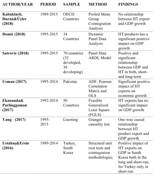
The extent literature reveals evidence of a causal link between exports and economic growth across many countries using different methodologies. In order to be consistent with the purpose of this study and to demonstrate the research gap in empirical literature, Table 1 below, lists research that has included high-tech products as a dependent variable and are included in the literature review. Table 1 includes a listing of authors, year of the publication, sample countries, methodologies and the key findings of the relevant literature.
Table 1. Literature Review
AUTHOR/YEAR PERIOD SAMPLE METHOD FINDINGS
Kabaklarlı, Duran&Üçler (2018)
1989-2015 OECD
Countries Pooled Mean Group Cointegration Analysis No relationship between HT export and GDP growth Demir (2018) 1995-2015 34
Countries Dynamic Panel Data Analysis HT products has a significant positive impact on GDP growth Satrovic (2018) 1995-2015 70 countries (32 developed, 38 developing) Panel Data
ARDL Model Positive and significant relationship between GDP and HT in both, short- and long-term
Usman (2017) 1995-2014 Pakistan ADF, Pearson
Correlation Matrix and OLS Significant positive impact of HT exports on economic growth Ekananda& Parlinggoman (2017) 1992-2014 50
Countries Feasible Generalized Least Square (FGLS) HT exports has no significant impact on GDP growth Yang (2017) 1995-
2015 Liaoning Granger causality test One-way causal relationship between HT product export and GDP growth
Ustabaş&Ersin
(2016) 1989-2014 Turkey, South
Korea
Structural unit root tests and cointegration methodologies
Positive impact of HT exports on GDP in South Korea both in the long and short-run, for Turkey only in short-run
Bal et al. (2016) 2013-2015 10 OECD
Countries System GMM Panel Estimator HT exports have positive and statistically significant impact on GDP growth Kılavuz&Topcu (2012) 1998-2006 22 Developing Countries Panel Data Analysis (OLS, RE, FE, PCSE methods)
HT export has a significant effect on GDP growth
Jarreau & Poncet
(2012) 1997-2009 China Cross-section analysis Regions that specialize in more
sophisticated goods subsequently grow faster
Yoo (2008) 1988-2000 91
Countries Cross-section analysis HT exports significantly contribute to GDP growth
Falk (2007) 1980-2004 22 OECD
Countries GMM Panel Estimator HT exports are significantly positively related to GDP growth
Source: Authors' own construction
2. Econometric Analysis
2.1. Data Set, Variables, Methodology
The dataset used in this study, which investigates the impact of high technology product exportation on economic growth, covers 450 observations composed of GDP, High-technology exports (HT), labor force (LF), Gross fixed capital formation (PC) of EU-15 countries, between 1998 -2017. The Dataset was compiled from the “World Bank”.
Primarily the functional, statistical and VAR models were established. Before proceeding with the long-term and the short-term analysis, a number of pre-tests are required to determine appropriate test methods. These tests are cross-section dependence, stationary of the series, homogeneity of the parameters. Before panel causality tests can be used, the stationary of the series as well as the integration levels needs to be determined. Because panel causality analysis using time-series data which are non-stationary, produces biased results. Moreover, determining integration levels of the series are as crucial as stationary of the series. Stationarity can be evaluated using a Unit Root Test. To decide which unit root test is the best to produce proper results, the existence of the correlation between the units should be tested. To test the correlation between the units, a cross section dependence test is employed. In case of the existence of
cross-section dependence, it is recommended to use one of the second-generation unit root test, otherwise the first-generation. In this research a Pesaran (2015) CD Test and Breusch Pagan LM Test were employed to test the existence of cross-section dependence. Pesaran (2007) CADF was implemented to define the stationary of the series.
Homogeneity of the parameters in another crucial pre-test to determine the proper estimation method. Therefore, Swamy S Homogeneity was conducted to determine the homogeneity of the parameters. Based on the pre-test mentioned above, the short-term causal relationship was analysed with the help of Dumitrescu & Hurlin (2012) Granger Panel Causality Test. Before examining the long-term relationship in detail, it is needed to determine the existence of cointegration between the series. For this purpose “Westerlund ECM Panel Co-integration Test” was employed. Finally, according to the results of the tests explained above Mean Group Estimator was chosen as the proper method to produce more detail in both the long-term and the short-term relationships,
2.2. Model
While examining the impact of high technology exports on economic growth, the equation based on the Cobb-Douglas function developed by Solow (1957), which is presented in Eq. (1), was implemented.
𝑌𝑌"= 𝐴𝐴 𝑡𝑡 𝐾𝐾"( 𝐿𝐿(+,()" (1)
Solow's equation can be expressed in logarithmic function form as in Eq.(2). 𝐿𝐿𝐿𝐿𝐿𝐿𝑌𝑌"= 𝐿𝐿𝐿𝐿𝐿𝐿𝐴𝐴 𝑡𝑡 + 𝛼𝛼𝐿𝐿𝐿𝐿𝐿𝐿𝐾𝐾 + 1 − 𝛼𝛼 𝐿𝐿𝐿𝐿𝐿𝐿𝐿𝐿 (2) Accordingly, the functional model that will be used in this study can be described as in Eq.(3). In the model, GDP represents the economic growth and is the predicted variable of the model, while High-technology exports (HT), labour force (LF), Gross fixed capital formation (PC) are the predictor variables of the model.
𝐺𝐺𝐺𝐺𝐺𝐺 = 𝑓𝑓 𝐻𝐻𝐻𝐻, 𝐿𝐿𝐿𝐿, 𝐺𝐺𝑃𝑃
GDP : Gross Domestic Product (constant 2010 US$) HT : High-technology exports (current US$) LF : Labour force
PC : Gross fixed capital formation (current US$)
(3)
Eq(2) can be expressed statistically as in Eq.(4)
In Eq.(4) where 𝑎𝑎 represents fixed term and 𝛽𝛽+, 𝛽𝛽@ 𝑎𝑎𝑎𝑎𝑎𝑎 𝛽𝛽A are the coefficients of the regression which indicates the sensitiveness of GDP corresponding with per unit change in HT, LF and PC respectively. 𝑡𝑡 symbolizes the time trend and 𝑢𝑢 is the error term, while 𝑖𝑖 represents countries(𝑖𝑖 = 1 … 𝑁𝑁).
The static model which is presented in Eq(4) can be described in dynamic equations in VAR System by considering lagged values of the series as in Eqs.(5), (6), (7) and (8) below. 𝑎𝑎𝑑𝑑𝑑𝑑𝑑𝑑"= 𝑎𝑎+++ IHJ+𝛽𝛽+H𝑎𝑎𝑑𝑑𝑑𝑑𝑑𝑑=",H+ IHJ+𝛽𝛽@H𝑎𝑎𝑑𝑑𝑑𝑑=",H+ IHJ+𝛽𝛽AH𝑎𝑎𝑑𝑑𝑑𝑑=",H+ IHJ+𝛽𝛽KH𝑎𝑎𝑑𝑑𝑑𝑑=",H+ 𝑢𝑢+" (5) 𝑎𝑎𝑑𝑑𝑑𝑑"= 𝑎𝑎@++ IHJ+𝛽𝛽LH𝑎𝑎𝑑𝑑𝑑𝑑=",H+ IHJ+𝛽𝛽MH𝑎𝑎𝑑𝑑𝑑𝑑𝑑𝑑=",H+ IHJ+𝛽𝛽NH𝑎𝑎𝑑𝑑𝑑𝑑=",H + IHJ+𝛽𝛽OH𝑎𝑎𝑑𝑑𝑑𝑑=",H 𝑢𝑢@" (6) 𝑎𝑎𝑑𝑑𝑑𝑑"= 𝑎𝑎A++ IHJ+𝛽𝛽PH𝑎𝑎𝑑𝑑𝑑𝑑=",H+ IHJ+𝛽𝛽+QH𝑎𝑎𝑑𝑑𝑑𝑑𝑑𝑑=",H+ IHJ+𝛽𝛽++H𝑎𝑎𝑑𝑑𝑑𝑑=",H+ 𝛽𝛽+@H𝑎𝑎𝑑𝑑𝑑𝑑=",H I HJ+ + 𝑢𝑢A" (7) 𝑎𝑎𝑑𝑑𝑑𝑑"= 𝑎𝑎K++ IHJ+𝛽𝛽+AH𝑎𝑎𝑑𝑑𝑑𝑑=",H+ IHJ+𝛽𝛽+KH𝑎𝑎𝑑𝑑𝑑𝑑𝑑𝑑=",H+ IHJ+𝛽𝛽+LH𝑎𝑎𝑑𝑑𝑑𝑑=",H+ 𝛽𝛽+MH𝑎𝑎𝑑𝑑𝑑𝑑=",H I HJ+ + 𝑢𝑢K" (8)
In the VAR Model, 𝑎𝑎 shows “the first differences”, 𝑢𝑢+", 𝑢𝑢@", 𝑢𝑢A" 𝑎𝑎𝑎𝑎𝑎𝑎 𝑢𝑢K" are the “error terms”, 𝑎𝑎 is “the number of lag-lengths” and 𝛽𝛽+H … 𝛽𝛽+MH are the coefficients of the model.
2.3. Cross-section Dependence Analysis
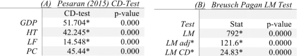
In order to define the right unit root test method as well as the right panel cointegration method, correlation between the units should be considered. In case the existence of cross-section dependence between the units, the second-generation panel unit root test, otherwise, the first-second-generation panel unit root test will be employed. Similarly, if there is a cross-sectional dependence between the units, the second-generation cointegration tests, if not, the first-generation cointegration tests should be used. "Pesaran (2015) CD Test and Breusch Pagan LM Test” are employed to determine the correlation between the units and the outcomes are presented in Table 2.
Table 2. CD-Test
(A) Pesaran (2015) CD-Test
CD-test p-value
GDP 51.704* 0.000
HT 42.245* 0.000
LF 14.548* 0.000
PC 45.44* 0.000
(B) Breusch Pagan LM Test Test Stat p-value
LM 792* 0.0000
LM adj* 121.6* 0.0000
LM CD* 24.83* 0.0000 Table 2A includes the CD test statistics, p-values of Pesaran (2015) Test. “H0: There is no correlation between the units” has been tested. As it is seen that all the p-values belong to GDP, HT, LF and PC are lower than 5% significance
level and therefore, “H0 is rejected”. Similarly, the p-values of the test statistics of Breusch Pagan LM Test, which are presented in Table 2B, are lower than 5%. Both methods produced the same result and concluded that there is a correlation between the units.
2.4. Stationarity Analysis
It is decided to employ Pesaran (2007) CADF test which is one of the second-generation unit root test that consider the correlation between the units. The outcomes of the test are presented in Table 3.
Table 3. Unit Root Test
t-bar cv10 cv5 cv1 Z[t-bar] P-value
GDPC -2.196 -2.140 -2.250 -2.450 -1.702 0.044 HT -2.213 -2.140 -2.250 -2.450 -1.767 0.044 PC -2.481 -2.140 -2.250 -2.450 -2.838 0.002 LF -2.392 -2.140 -2.250 -2.450 -2.482 0.007
The outcomes of the test shown in Table 3 indicates that GDP, HT, PC and LF are stationary at level since the p-values of Z [t-bar] statistics belong to the series are lower than 5%. In other words, the integration orders of the series are I(0).
2.5. Homogeneity Analysis
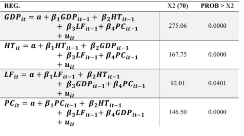
Determining the heterogeneity or homogeneity of the parameters is crucial issue in order to define the right panel causality method. Accordingly, Swamy S Homogeneity Test was implemented and the outcomes are presented in Table 4.
Table 4. Homogeneity Test
REG. Χ2 (70) PROB > Χ2 𝑮𝑮𝑮𝑮𝑮𝑮𝒊𝒊𝒊𝒊 = 𝒂𝒂 + 𝜷𝜷𝟏𝟏𝑮𝑮𝑮𝑮𝑮𝑮𝒊𝒊𝒊𝒊,𝟏𝟏+ 𝜷𝜷𝟐𝟐𝑯𝑯𝑯𝑯𝒊𝒊𝒊𝒊,𝟏𝟏 + 𝜷𝜷𝟑𝟑𝑳𝑳𝑳𝑳𝒊𝒊𝒊𝒊,𝟏𝟏+ 𝜷𝜷𝟒𝟒𝑮𝑮𝑷𝑷𝒊𝒊𝒊𝒊,𝟏𝟏 + 𝒖𝒖𝒊𝒊𝒊𝒊 275.06 0.0000 𝑯𝑯𝑯𝑯𝒊𝒊𝒊𝒊= 𝒂𝒂 + 𝜷𝜷𝟏𝟏𝑯𝑯𝑯𝑯𝒊𝒊𝒊𝒊,𝟏𝟏+ 𝜷𝜷𝟐𝟐𝑮𝑮𝑮𝑮𝑮𝑮𝒊𝒊𝒊𝒊,𝟏𝟏 + 𝜷𝜷𝟑𝟑𝑳𝑳𝑳𝑳𝒊𝒊𝒊𝒊,𝟏𝟏+ 𝜷𝜷𝟒𝟒𝑮𝑮𝑷𝑷𝒊𝒊𝒊𝒊,𝟏𝟏 + 𝒖𝒖𝒊𝒊𝒊𝒊 167.75 0.0000 𝑳𝑳𝑳𝑳𝒊𝒊𝒊𝒊 = 𝒂𝒂 + 𝜷𝜷𝟏𝟏𝑳𝑳𝑳𝑳𝒊𝒊𝒊𝒊,𝟏𝟏+ 𝜷𝜷𝟐𝟐𝑯𝑯𝑯𝑯𝒊𝒊𝒊𝒊,𝟏𝟏 + 𝜷𝜷𝟑𝟑𝑮𝑮𝑮𝑮𝑮𝑮𝒊𝒊𝒊𝒊,𝟏𝟏+ 𝜷𝜷𝟒𝟒𝑮𝑮𝑷𝑷𝒊𝒊𝒊𝒊,𝟏𝟏 + 𝒖𝒖𝒊𝒊𝒊𝒊 92.01 0.0401 𝑮𝑮𝑷𝑷𝒊𝒊𝒊𝒊 = 𝒂𝒂 + 𝜷𝜷𝟏𝟏𝑮𝑮𝑷𝑷𝒊𝒊𝒊𝒊,𝟏𝟏+ 𝜷𝜷𝟐𝟐𝑯𝑯𝑯𝑯𝒊𝒊𝒊𝒊,𝟏𝟏 + 𝜷𝜷𝟑𝟑𝑳𝑳𝑳𝑳𝒊𝒊𝒊𝒊,𝟏𝟏+ 𝜷𝜷𝟒𝟒𝑮𝑮𝑮𝑮𝑮𝑮𝒊𝒊𝒊𝒊,𝟏𝟏 + 𝒖𝒖𝒊𝒊𝒊𝒊 146.50 0.0000
Table 5 shows the χ2 (70) and Prob. values of χ2 of the regressions which are seen in the first column of the table. "H0: parameters are homogeneous” is
tested against the parameters are heterogeneous. Because all Prob > χ2 are less than 0.05, H0 was rejected and concluded that parameters are heterogeneous,
therefore, heterogeneous panel causality and heterogeneous cointegration methods should be implemented.
2.6. Short-Term Causality Analysis
In the short-term causality analysis between the series, Dumitrescu & Hurlin (2012) Granger Panel Causality Test, which takes into account the heterogeneity, is employed and the outcomes are shown in Table 5.
Table 5. VAR Panel Causality Test Results
H0 : W-bar Stat. Z-bar Stat. (p-value) Relationships
HT ⇏ GDP 12.5129 4.3696 (0.0000) HT
↔
GDP GDP ⇏ HT 21.4775 13.0496 (0.0000) LF ⇏ GDP 12.4541 4.3127 (0.0000) LF↔
GDP GDP ⇏ LF 21.5863 13.1549 (0.0000) PC ⇏ GDP 20.6877 12.2848 (0.0000) PC↔
GDP GDP ⇏ PC 30.1492 21.4459 (0.0000) PC ⇏ HT 9.0632 1.0294 (0.3033) PC←
HT HT ⇏ PC 18.3215 9.9937 (0.0000) LF ⇏ HT 17.0922 8.8035 (0.0000) LF↔
HT HT ⇏ LF 10.3056 2.2324 (0.0256) LF ⇏ PC 19.2849 10.9265 (0.0000) LF↔
PC PC ⇏ LF 19.2169 10.8607 (0.0000)Note: (⇏) refers “does not Granger-cause”
Dumitrescu & Hurlin (2012) Granger Panel Causality Test Results, which are seen in Table 6, indicated:
(a) a two-way causality between HT and GDP, (b) a two-way causality between LF and GDP, (c) a two-way causality between PC and GDP, (d) a one-way causality from HT to PC, (e) a two-way causality between LF and HT, (f) a two-way causality between LF and PC.
2.7. Long-term Analysis
Existence of long-term relationships were investigated with the help of “Westerlund ECM Panel Co-integration Test”, which is one of the second-generation cointegration test method that considers cross-section dependence between the units and the heterogeneity of the parameters. The outcomes of the test are presented in Table 6.
Table 6. Westerlund ECM Panel Co-integration Outcomes
Statistic Value z-value P-value Robust P-value
Gt -2.680** -3.670 0.000 0.030 Ga -9.002** -0.739 0.230 0.040 Pt -10.782** -4.335 0.000 0.030 Pa -11.765* -4.597 0.000 0.000 Note: ** and * indicate cointegration at the 5% and 1% significance level respectively.
Table 7 displays the values of test statistics, z-values, p-values and robust p-values of Gt, Ga, Pt and Pa. “H0: no cointegration hypothesis” was tested.
Since the robust p-values of Gt, Ga, Pa, which are considered in heterogeneous panel cointegration, are less than 5% the significance level, “The null hypothesis is rejected” and therefore it is concluded existence of co-integration between the units.
Because of the outcomes of Table 6 confirmed a long-term relationship, Mean Group Estimator is employed to get more detail. The outcomes of the MG Estimator are presented in Table 7.
Table 7. MG Estimator Outcomes
dLnGDP Coef. Std.Err. z P > I z I [%95 Conf. Interval] _ec L.LnHT L.LnLF L.LnPC .3373107 7.399851 .3261508 .0879829 3.659781 .1172043 3.83 2.02 2.78 0.000 0.043 0.024 .1648675 .2268113 .4558671 .509754 14.57289 .0035655 SR _ec -.1636886 .0613012 2.67 0.008 -.2838367 -.0435406 d.LnHT .48686 .0154644 3.15 0.002 .0183764 .0789956 d.LnLF .2207495 .1917353 1.15 0.250 -.1550447 .5965437 d.LnPC .0480197 .0130922 3.67 0.000 .0223594 .0736799 d.L.LnGDP .1183899 .0833607 1.42 0.156 -.044994 .2817738 d.L.LnHT -.0231869 .010314 -2.25 0.025 -.043402 -.0029718 d.L.LnLF -.0561468 .1153639 -0.49 0.626 -.2822559 .1699623 d.L.LnPC .0025046 .0093701 0.27 0.789 -.0158605 .0208698 _cons 1.904871 1.82685 1.04 0.297 -1.67569 5.485432
Table 7 displays the outcomes of MG Estimator and includes the long-term and the short-term coefficients, standard errors, z-values, p-values and 95% confident intervals.
The upper part of the Table 8 shows the long-term relationships. Since the p-values are lower than 0.05, the long-term coefficients of the variables are considered to be significant. Taking into account the long-term coefficients, it is deduced that:
(a) a 1% raise in HT causes a 0.34 % increase in GDP (b) a 1% raise in LF causes a 7,4 % increase in GDP, (c) a 1% raise in PC causes a 0.33% increase in GDP.
As a result, high-tech exportation, labour force and physical capital have a significant positive impact on economic growth in the long- term.
The second part of the outcomes of the MG Estimator show the short-term relationship. The coefficient of error correction (EC) is negative and p-value of (ec) is 0.008. Therefore, the short-term relationships are significant at 1% level. Considering the short-term coefficients belong to HT, LF and PC it is concluded that:
(a) a 1% raise in HT causes 0.49 % increase in GDP, (b) a 1% raise in LF causes 0.22 % increase in GDP, (c) a 1% raise in PC causes 0.48 % increase in GDP,
(d) Although LC itself does not appear significant in the short term (because of the interaction between the HT, LF and PC), the effect of the variables on economic growth in the short-term is positive and significant. (e) Approximately 16% of the imbalances in a period, because of a shock,
can be recovered in the next period. Conclusion
In this paper, the long-term and the short-term relationships between high-tech exportation and economic growth in EU-15 countries were examined. The dataset includes 450 observations from 1988 to 2017 composed of the variables gross domestic product (GDP), high-tech exports (HT), labour force (LF) and gross fixed capital formation (PC).
To reveal short-term causality between the series a Dumitrescu & Hurlin (2012) Granger Panel Causality Test, which takes into account the heterogeneity was performed. To discover the long-term relationships, Westerlund ECM Panel Cointegration Test and MG Estimator were used.
The results of the short-term Granger causal analysis revealed a bidirectional causal relationship between (a) HT and GDP, (b) LF and GDP, (c) PC and GDP, (d) LF and HT, (e) LF and PC, and (f) a unidirectional causality from HT to PC. The short-term outcomes of MG Estimator show that: (1) a 1% raise in HT cause to 0.049 % increase in GDP, (2) a 1% raise in LF cause to 0,22 % increase in GDP, (3) a 1% raise in PC cause to 0,48 % increase in GDP, (4) approximately 16% of the imbalances in a period, because of a shock, can be recovered in the next period. Although LF itself does not appear significant in the short term; however because of the interaction between the HT, LF and PC, the effect of the variables on economic growth in the short-term is positive and significant.
The long term results indicate that (1) a 1% raise in HT cause to a 0.34 % increase in GDP, (2) a 1% raise in LF cause to a 7,4 % increase in GDP, (3) a 1% raise in PC cause to a 0.33% increase in GDP.
The empirical findings of this study can be interpreted as follows. High-tech exportation has a significant impact not only on economic growth, but also on gross fix capital formation and employment. The magnitude of the impact of high-tech export is stronger in the long-term compared to short-term. This confirms that high-export exportation has the potential to increase the long-term growth, boosting the productive capacity in EU-15 countries. Results of the study supports the findings of Demir (2018), Satrovic (2018), Usman (2017), Bal et al. (2016), Kılavuz and Topcu (2012), Yoo (2008) and Falk (2007) who found the importance of high-tech exports on economic growth.
This study also revealed the importance of export diversification and product sophistication. Bidirectional causal relationship between high-tech product export and economic growth shows that the economic policies in EU-15 countries should promote both manufacturing and exportation of high-tech products and also activities that support economic growth. The findings of this study are applicable to countries where the share of high-tech product export is high. Further research is recommended for the rest of the EU countries to examine the impact across a broader range of economies.
REFERENCES
BAL, Harun, ÇİFTÇİ, Hakkı, İŞCAN, Erhan & SERİN, Duygu (2016), “The Export-Led Growth: A Technological View”, Proceedings from International Conference on Eurasian Economies 2016, session 5B: International Trade, pp. 311-316, Kaposvar.
CUARESMA, Jesus Crespo & WÖRZ, Julia (2005), “On Export Composition and Growth”, Review of World Economics, vol. 141, no. 1, pp. 33-49. DEMİR, Oguz (2018), “Does High Tech Exports Really Matter for Economic
Growth A Panel Approach for Upper Middle-Income Economies”, Online Academic Journal of Information Technology, vol. 9, no. 30, pp. 43-54. DUDZEVIČIŪTE, Gitana, ŠIMELYTE, Agne & ANTANAVIČIENĖ, Jūratė
(2017), “Causal Nexus Between Export and Economic Growth in the European Union Countries”, Montenegrin Journal of Economics, vol. 13, no. 2, pp. 107-120.
DUMITRESCU, Elena & HURLIN, Christophe (2012), “Testing for Granger Non-causality in Heterogeneous Panels”, Economic Modelling, vol. 29, no. 4, pp. 1450-1460.
EKANANDA, Mahjus & PARLINGGOMAN, Dion Jogi (2017), “The Role of High-Tech Exports and of Foreign Direct Investments (FDI) on Economic Growth”, European Research Studies Journal, vol. 20, no. 4A, pp. 194-212.
FALK, Martin (2007), “High-Tech Exports And Economic Growth in Industrialized Countries”, Applied Economics Letters, vol. 16, no. 10, pp. 1025-1028.
HAUSMANN, Ricardo & KLINGER, Bailey (2006), “Structural Transformation and Patterns of Comparative Advantage in the Product Space”, Harvard University Faculty Research Working Papers Series No. RWP06-041. JARREAU, Joachim & PONCET, Sandra (2012), “Export Sophistication and
Economic Growth: Evidence from China”, Journal of Development Economics, vol. 97, no. 2, pp. 281-292.
KABAKLARLI, Esra., DURAN, Mahmut Sami & ÜÇLER, Yasemin Telli (2018), “High-Technology Exports and Economic Growth: Panel Data Analysis for Selected OECD Countries”, Forum Scientiae Oeconomia, vol. 6, no. 2, pp. 47-60.
KILAVUZ, Emine & TOPCU, Altay (2012), “Export and Economic Growth in the Case of the Manufacturing Industry: Panel Data Analysis of Developing Countries”, International Journal of Economics and Financial, Vol. 2, No. 2, 2012, pp. 201-215.
OECD (2011), “ISIC REV.3 Technologhy Intensity Definition: Classification of Manufacturing Industries into Categories Based on R&D Intensities”, OECD Directorate for Science, Technology and Industry Economic Analysis and Statistics Division.
PESARAN, M. Hashem (2007), “A Simple Panel Unit Root Test in The Presence of Cross-Section Dependence”, Journal of Applied Econometrics, vol. 22, no. 2, pp. 265– 312.
PESARAN, M. Hashem (2015), “Testing Weak Cross-Sectional Dependence in Large Panels”, Econometric Reviews, vol. 34, no. 6-10, pp.1088–1116. SATROVIC, Elma (2018), “Economic Output and High-Technology Export:
Panel Causality Analysis”, International Journal of Economic Studies, vol. 4, no. 3, pp. 55-63.
SCHOTT, Peter K. (2004), “Across-Product versus Within-Product Specialization in International Trade”, The Quarterly Journal of Economics, vol. 119, no. 2, pp. 646-677.
SOLLOW, Robert (1957), “Technical Change and the Aggregate Production Function”, Review of Economics and Statistics, vol.39, pp. 312-320. TYTELL, Irina, EMSBO-MATTINGLY, Lisa & HOFSCHIRE, Dirk (2018),
Secular Outlook for Global Growth: The Next 20 Years, Fidelity Investments Leadership Series, https://institutional.fidelity.com/app/proxy/content?literatureURL=/95954 6.PDF, Online: 15.05.2019
USMAN, Muhammad (2017), “Impact Of High-Tech Exports on Economic Growth: Empirical Evidence from Pakistan”, RISUS - Journal on Innovation and Sustainability, vol. 8, no. 1, pp. 91-105.
USTABAŞ, Ayfer & ERSİN, Özgür Ömer (2016), “The Effects of R&D and High Technology Exports on Economic Growth: A Comparative Cointegration Analysis for Turkey and South Korea”, Proceedings from International Conference on Eurasian Economies 2016, session 2A: Growth, pp. 44-55, Kaposvar.
WORLD BANK (2018), World Development Indicators, Washington, D.C.: The World Bank.
YANG, Feixue (2017), “The Positive Influence of High-tech Product Export on Economic Growth in Liaoning Province”, Journal of Simulation, vol. 5, no. 4, pp. 7-9.
YOO, Seung-Hoo (2008), “High-Technology Exports and Economic Output: An Empirical Investigation”, Applied Economics Letters, vol. 15, no. 7, pp. 523-525.