Reconstruction of time series data wİth missing values

(1)

J

oumal of Applied Seienees

7 (6): 922-925, 2007

ISSN

1812-5654

©

2007

Asİan Network for Scientific Information

Reconstructİon of Time Series Data wİth Missing Values

Mitat Uysal

Dogus University, Aeibadem-Kadikoy

34722,

Istanbul, Turkey

Abstract: Missing data are a part of almüst all research and it must be decided how to dea! with it from time to time. Missing data creates several problems İn many applications which depend on good access to accurated data. Conventiona! methods for missing data, like listwİse deletion or regression imputation, are prone to three serİolis problems: Inefficİent use of the available information, leading to low power and Type II errüfS. Biased estimates of standard errüfS, leading to İncorrect p-values. Biased parameter estimates, due to failure to adjust for selectivity İn missing data. In this study, we propose a new algorithrn to predict missing values of a given time series using Radial Basis Fwıctions.

Key words: Handling missing data, time series, radial basis fwıctions, fwıction approximation, forecasting modeling, simulation

INTRODUCTION

Time series data are used to represent many real world phenomenon. For various reasons, a time series database may have some missing data. Traditional interpolation or estimation methods usually become invalid when the observation interval of the missing data is not small (Hong and Chen,

2003).

The methods of handling missing data are direetly related to the mechanisms that cmısed the incompleteness. These mechanisms fall into three classes (Sentas and Angelis,

2005;

Little and Rubin,

2002).

• Missing Completely at Random (MCAR): The

missing value s in a variable are wrrelated to the values of any other variables, whether missing or valid.

• Non-Ignorable Missingness (NIM): The probability

of having missing values in a variable depends on the variable itself.

• Missing at Random (1.1AR): This can be considered

as an intermediate situation between MCAR and NIM. The probability of having missing values, does not depend on the variable itself but on the values of some other variable.

Missing data techniques are given in Little and Rubin

(2002).

They can be listed as: Listwise deletion, mean imputation, regression imputation and expectation maximization. Details can be obtained from Little and Rubin

(2002).

Many recent publications appeared in literature related to dealing missing data.

922

Choi and Kim

(2002)

presented a physies-based approach for automaticaııy reconstructing three dimensional shapes in a robust and proper manner from partiaııy missing data.

Tang and Hung

(2006)

have proposed an algoritbm to estimate projective shape, projective depths and missing data iteratively.

Yemez and Wetherilt

(2007)

presented a hybrid surface reconstruction method that fuses geometrical information acquired from silhouette images and optical triangulation.

Golyandina and Osipov

(2007)

have proposed a method of fiııing in the missing data and applied to time series of finite rank.

Heintzmann

(2007)

introdueed a novel way of measuring the regain of out-of-band information during maximum likelihood deconvolution and applied to various situations.

Formal representation of missing data: Original data matrix D �

(d,,)

i �

1 ,2,3

... n, j �

1,2,

... k eontains time series

data where d,J is the value of variable � for case 1. When there are missing data, the missing data indicator matrix M = (m,) can be defined as below:

if m'J =

1

then d,J is missing

if m'J =

O

then d,J is present

(Sentas and Angelis,

2005).

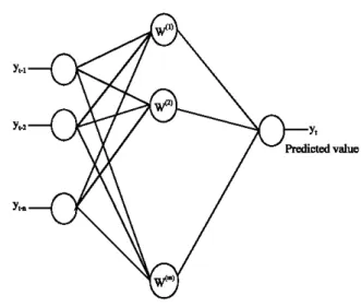
Radial basis funetions for time series forecasting: An RBF network consists of

3

layers: an input layer, a hidden layer and an output layer. A typical RBF network is shown in Fig.

1.

Mathematically, the network output for linear output nodes can be expressed as below:

(2)

J. Applied Sci .•

7 (6): 922-925. 2007

Fig. i: Typical RBF network

h(x)

�

i:

w k,<D,

(ii

x - x,

ii)

+ w kC J�ı

Where x İs the input vector with elements X, (where i İs the dimensİon of the input vector),

xJ İs the vector to determine the center of the basİs fwıction <L>J with elements XJ!, wlg 's are the weights and WkC is the bias (Haıpham and Dawson.

2006).

The basis fwıction <L>J (

-)

provides the nonlinearity. The most used basİs fimctions are Gaussİan and multiquadratic [wıctions (Haıpham and Dawson,

2006).

Calculating the optimal values of weights: A very important property of the RBF Network İs that it İs a linearly weigthed network in the sense that the output İs a linear combination of ın radial basİs [wıctions, wrİtten

as below:

m

[(x)

� L:

WC')<DC') (x) ,�ı

(Duy and Chong,

2003)

The main problem İs to [ind the wıknown weights {w(I)

}

1= ı

,

m For this purpose, the general least squares

principle can be used to minimİze the surn squared error:

" _,

SSE � L:[

y") - [(xC,))

J

1=1

With respect to the weights of f, resulting in a set of m sirnultaneous linear algebraic equations in the m urıkno\VIl weights

(BTB)w � BTy

923

Fig.

2:

Finding the predicted value y, where

<D0)(XO)) <Dc,)(xO))

B�

<D0)(xC')) <Dc,)(xC'))

<DCm)(XO)) <DCm) (xC'))

In the special case where n = m the resultant system is

just

Bw�y (Duy and Chong,

2003)

The output y(x) represents the next value of Y in time t taking input values x), Xb ... Xı, that represent the previous fwıction values set of the time series with values Yı.j, Yı.b ... Yı.n· So, xı, corresponds to yı.), Xı,.ı corresponds to Yı.2 etc. as in Fig.

2.

Reconstruetion of data series by radial basis funetions: a new algorithm: The following algorithrn is proposed in this work to find the values of missing data.

• Remove the

20%

of the original data from the data

set. Divide the data set into segments so that each segment contains some missing data:

compıeıe_

�

M;"mg_

.. 1

. .

\

. .

1

. .

1

. .

1

. . . . .

.

. . .

111 ...

. .

(3)

J. Applied Sci .•

7 (6): 922-925. 2007

• Use the complete data of segmen� to [ind an artificİa!

time series equation with an RBF network that means [incling the weights in the RBF approximation.

• Calculate the error İn each segment according to the

following formula:

Where ei İs the error value in the � point on the

/'

segment.

• Calculate the surn squared errüfS in each segment İn

each pass of the algoritlnn.

SSEk �

L2

)e,')'

J=l 1=1

where k İs the number of the pass.

• Replace the missing data with the predicted values İn

each segment İn the pass ın where SEEm İs the

minimum value of SSEk. Stop the algoritlnn.

SIMULA TION RESUL TS

Several simulation

nıns

were carrİed out İn a computer envİrornnent to [ind the optimal values of parameters in radial basİs flUletiorn like width

ö

and centers

(xı

Ps

)

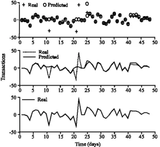
to obtaİn good predictions for the missing data İn the time series.

Figure

3

shows the results of the first simulation nm.

In this

fULL,

the first 40 data items were used to predict the next

8

data items that was considered missing data and the results were compared with the real data. Real

so

+ Real O Predicted + O -50

+-__,_-r_--,----,--r-�-.._____,_-r__,

O 5 10 15 20 25 30 35 40 45 50

ı:ı=�

-50 O

_{5 10}

l'

40

4

5 5

0

S

:ı-

Real -50 O

_{5 10}

1'

2

0 2

5 3

0 3

5

40

4

5 5

rnne (w.y,)

Fig.

3:

Gaussian FlUlction sigma =

0.93

and

18

neurons in

the hidden layer

9

2

4

50 + Real O Predicted + O

O

..

_•

"..�.--IJ ff1Jfa�"e .. ·.ILIiIiLıı ...

_...-e.

_ii

_.,

_.ee

+ + -50

+---,---r---,---r---,---r----r--r----r---,

0 5 10 15 20 25 30 35 40 45 �

--

Predic100

.g

�

O • i

�

lı

50

ı·_···

_Real -50 O

₅

1

0 l

5 2' 0 2

5 3

0 3

5 4

0 4' 5

is

_2' ₀ ₂

_{5 3}

_{0 3}

₅

Jo

_4' _S

Thne (w.y,)

50 5

0

Fig.4: Gaussian FlUlction sigma =

1

and

18

neurons in

the hidden layer 20 + Real O Predicted O

tOeôOo6�'

t

�

0 ••

0$' .$�$t�O�e�Ô

�

$

t ,O t

iıo

Ot

-20 -40

t

285 290 295 300 305 310 315 320 325 20 ••••

_--

_...

Real Predicted

§

O

.�

-20

�

-40 285 290 295 300 305 310 315 320 325 20

--

_Real O -20 -40+--r--,---,---,----,---r-,----, 285 290 295 300 305 310 315 320 325

rnne (w.y,)

Fig.

5:

Gaussian FlUlction sigma =

1

and

18

neurons in the

hidden layer for the las! 40 data

data values are represented with symbol + and predicted values are represented with symbol o.

In Fig. 4, similar experiment was carried out with

Ö

=

1

for a Gaussian flUlction and better results

were obtained.

Figure

5

shows, the results of the similar experiment for the last 40 data items for a Gaussian flUlction.

(4)

J. Applied Sci .•

7 (6): 922-925. 2007

CONCLUSIONS

In this study,

i

proposed a new algorithrn to predict

missing values of a given time series using Radial Basİs

Fwıctions. Radial Basİs FlUlCtiOllS provide a good way to

predict the value s of missing data İn a time series. In this

study, a münthly data log of a bank was used to carry out

the sİmulation experiments. The data log file consİsted of

324 data items. This file was divided to small parts with 48

data items for the first 6 parts and 36 data items for the last

part. The last 20% of the data for each part was removed

and these removed data items were predicted using RBF's

and the 80% of the data items for each part. For some

optimal parameters of the RBF's, very good predictions

are obtained for the missing data.

REFERENCES