A microeconometric analysis of household consumption expenditure determinants for both rural and urban areas in Turkey

American International Journal of Contemporary Research Vol. 2 No. 2; February 2012

A Microeconometric Analysis of Household Consumption Expenditure

Determinants for Both Rural and Urban Areas in Turkey

Department of Econometrics

Faculty of Economics and Administrative Sciences Marmara University, Istanbul, Turkey

&

Department of Economics

Faculty of Economics and Administrative Sciences Turkey Manas University

Bishkek, Kyrgyzstan.

Melek ASTAR

Lecturer

Istanbul Bilim University Istanbul, Turkey

Abstract

This paper investigates the determinants of household consumption expenditure in Turkey. It also estimates the models for both rural and urban areas separately to examine the regional gaps for the entire distribution of consumption expenditure. Quantile regression is used to examine the correlates of consumption at different point on the distribution for both rural and urban areas. The findings show that the age increases the consumption expenditures in general and urban estimations, while it decreases the consumption expenditures in the rural estimations. In rural estimates, only age, income, marital status, insurance and the size of the household are obtained significantly. In the estimates through all observations regardless of rural-urban distinction, the lower value of consumption expenditures of men than the consumption expenditures of women are rather close to the values obtained for the same variables in the urban estimates.

Key words: household consumption, rural area, urban area, quantile regression Jel classification: O18; O50; C21

1. Introduction

Individual consumer behaviors make up the foundation of traditional demand theory. For this reason, the importance given to the accurate analysis of individual consumer behaviors considered as the foundation of the microeconomy has risen significantly in the recent years. The consumer theory examines the consumer decisions made by the consumers in a certain period of time and the direction of these decisions. This theory may easily reach the data of household consumption expenditures of states and can be analyzed with various aspects and the information about the consumer decisions are gathered as a result of these analyses. The purchase decisions of the consumers are affected by various factors. Income, prices, distribution of income, educational status of the individuals, occupation, age, and socio-cultural factors are the main ones. Besides these factors, the welfare of the consumer is enhanced when the consumer maximizes the benefit by giving priority to the purchase of the goods and services that avails the most and putting off purchasing the least needed goods and services due to income-bound. Thus, differences emerge according to the consumer behaviors and the effects of the factors determining these behaviors. The analysis of consumer behaviors enables the following of both social and demographic factors along with the changes in the cultural structure, and development of policies as a result of these impressions. For this reason, household consumption expenditures have a significant and vast place in the literature.

When the studies about the sub-groups of consumption expenditures are examined, the data gathered with the total consumption expenditures are generally about the sub-groups constituting the quantiles of total consumption expenditures. For this reason, this study aims to determine the factors affecting total household consumption expenditures in Turkey.

For this purpose, as in the studies examining the household consumption expenditures, it is not possible to model all the information about the persons in the household, so on behalf of the household, the demographic data such as education, age, gender, marital status of household head are examined. Quantile regression is used to determine the effects of factors effecting consumption expenditures on low and high quantiles. The reason of the use of this regression is to observe the response of the consumption expenditures against the change in the aforementioned factors in different points. The remainder of the paper organized as follows: The following section is including introduction. Sections 2 and 3 present the literature about the household consumption expenditures and quantile regression, respectively. The data and variables are introduced in Section 4. Section 5 reports the estimation results. Finally we present some concluding remarks in Section 6.

2. Earlier Studies

When the literature about the household consumption expenditures is examined, it is observed that analyses in terms of the expenditure groups are generally included. Moreover, also some studies examining the consumption expenditures according to urban-rural distinction are included. Burney et al. (1991) examined the household expenditures in Pakistani in the period 1984-1985 with OLS considering the Engel curve. Rural and urban areas are approached separately in the study, and there are some interpretations in the study indicating that the consumption expenditures in the urban areas are higher than the consumption expenditures in the rural areas according to Engel law. Qu and Zhao (2008) examined the inequality between the consumption expenditures in the rural and urban areas in the period 1988-2002 for China with quantile regression. It is underlined in the study that price effect is crucial for inequality and rural education must be developed to decrease this inequality by drawing attention to inequality between the rural and urban areas. Nguyen et al. (2006) examined the welfare inequality between urban and rural areas with quantile regression in their study about the period 1993-1998 for Vietnam. Household consumption expenditures are considered as a standard in this study, and it is stated that the differences in the variables of education, ethnicity and age have influence on the rural-urban distinction. Ranning and Schulze (2004) examined the household beer and wine consumption expenditures for Germany with both OLS and quantile regression. The results obtained are interpreted with the price elasticity for household beer and wine consumption.

3. Quantile Regression

Quantile regression introduced by Koenker and Basset (1978) is a method to estimate the conditional of a variable. This regression has the potential of generating different responses in the dependent variable at different quantiles. These different responses may be interpreted as differences in the response of the dependent variable to changes in the regressors at various points in the conditional distribution of the dependent variable (Montenegro 2001).

Quantile regression models assume that the conditional quantile of a random variable Y is a linear in the regressors X,

Yi = Xiβθ+ εθi with Quantθ Yi Xi = Xiβθ (2)

where Xi is the vector of independent variables and βθ is the vector of parameters. Quantθ Y X is the θth

conditional quantile of Y given X. Estimation of the quantile parameters is performed as the solution to

min_β∈Rk i:Yi>Xiβθ Y_i− X_iβ_θ + _i:Yi<Xiβ(1 − θ) Y_i− X_iβ_θ . (3)

Standard errors for the vector of parameters are obtainable by using the bootstrap method described in Buchinsky (1998). The quantile regression can provide a more complete description of the underlying conditional distribution compared to other mean-based estimators such as OLS.

4. Data

This study aims to determine the factors affecting the consumption expenditures for Turkey. The household consumption expenditures data gathered from Turkish Statistical Institute (TurkStat) in 2009 is used for the analysis. The data obtained from the household budget survey including 5658 sample households in the period January1-December 31, 2009 (TurkStat 2009-CD)1.

1

American International Journal of Contemporary Research Vol. 2 No. 2; February 2012

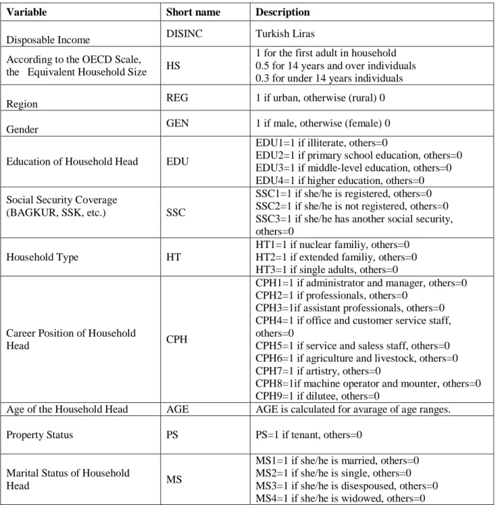
In the cross-section data obtained, after making necessary arrangements (missing observation, determination of socio-demographic features of household head instead of all persons in the household etc.) dummy variables are formed for independent variables. Dependent variable in the analysis is the total consumption expenditures determined as the total of main consumption preferences composed of 12 groups. The mathematical relation used to explain the relation between the consumption expenditures and the household forms the consumption functions. These functions can be formed between the income and total consumption expenditures as they can be formed between the household and single expenditure groups. Moreover, for the estimation of these consumption functions, the most appropriate functional form for the relation must be determined. The most commonly used ones are: linear, semi logarithmic, logarithmic and Working-Leser model. The estimates are formed with semilogarithmic form model in our study. For this reason, the logarithm of the dependent variable signifying total expenditure is included in the analysis. The definitions about the independent variables used in the model estimation are in the Table 1.

Table 1. Description of Independent Variables

Variable Short name Description

Disposable Income DISINC Turkish Liras

According to the OECD Scale,

the Equivalent Household Size HS

1 for the first adult in household 0.5 for 14 years and over individuals 0.3 for under 14 years individuals

Region REG 1 if urban, otherwise (rural) 0

Gender GEN 1 if male, otherwise (female) 0

Education of Household Head EDU

EDU1=1 if illiterate, others=0

EDU2=1 if primary school education, others=0 EDU3=1 if middle-level education, others=0 EDU4=1 if higher education, others=0 Social Security Coverage

(BAGKUR, SSK, etc.) SSC

SSC1=1 if she/he is registered, others=0 SSC2=1 if she/he is not registered, others=0 SSC3=1 if she/he has another social security, others=0

Household Type HT

HT1=1 if nuclear familiy, others=0 HT2=1 if extended familiy, others=0 HT3=1 if single adults, others=0

Career Position of Household

Head CPH

CPH1=1 if administrator and manager, others=0 CPH2=1 if professionals, others=0

CPH3=1if assistant professionals, others=0 CPH4=1 if office and customer service staff, others=0

CPH5=1 if service and saless staff, others=0 CPH6=1 if agriculture and livestock, others=0 CPH7=1 if artistry, others=0

CPH8=1if machine operator and mounter, others=0 CPH9=1 if dilutee, others=0

Age of the Household Head AGE AGE is calculated for avarage of age ranges.

Property Status PS PS=1 if tenant, others=0

Marital Status of Household

Head MS

MS1=1 if she/he is married, others=0 MS2=1 if she/he is single, others=0 MS3=1 if she/he is disespoused, others=0 MS4=1 if she/he is widowed, others=0

The education variable considered to affect the consumption pattern is defined with 4 dummy variables, i.e. illiterate, primary education, secondary education and higher education. The age variable having a significant effect on the welfare comparisons is formed by calculating the average of age groups of the household head. The gender, marital status, occupation and job status variables of the household head considered to play a key role in the expenditures of the household and the distribution of the expenditures are included in the analysis with the dummy variables. The marital status is formed with 4 dummy variables, i.e. married, single, widowed and divorced. With the thought that there may be consumption habits and differences, urban-rural distinction is included in the estimations using the region of the household as a base. For this reason, region dummy variable is formed signifying this region2. The ownership status of the household is dealt in terms of house savings models. For this reason, a dummy variable is defined not as the landlord for the payment status of rent, but as the landlord for the nonpayment status. The equivalence scale defined by OECD is used for the size of household3. This scale considers the 1 parameter for the first adult, 0,5 parameter for the individuals 14 years old or older, and 0,3 parameter for the individuals under 14 years old.

As the consumption functions are estimated with logarithmic linear models in our study, the functional model is taken into consideration for the parameter interpretations. The constant explanatory variables are interpreted by being multiplied by 100 in the models. The interpretation of the dummy variables is made according to Kennedy approach. Kennedy (1981) criticized the Halvorsen Palmquist (1980) approach commonly preferred in the literature for getting deviant results. The Kennedy approach gives less deviant results than Halvorsen Palmquist. According to Kennedy approach, the quantile effect of dummy variables on the dependent variable is calculated as follows:

𝑃 𝑘 = 100 𝑒

𝛽 −𝑉 𝛽₂

− 1 Here, 𝛽 is the parameter of dummy variable, and 𝑉 𝛽 is the variance of 𝛽 .

5. Empirical Findings

To determine the factors affecting the household consumption expenditures, three quantile regressions are estimated separately in our study. The form of the estimated quantile regression is

Quant (Yi | Xi) = Xi  + i

Where Y is the logarithmic consumption expenditure, X is the vector of independent variables. θ is the quantile being analyzed. We analyze conditional consumption expenditure at 9 representative quantiles: .10, .20, .30, .40, .50, .60, .70, .80, .90 which we will denote by Q10... Q50… and Q90, henceforth.

Firstly, the quantile regression model is estimated through the use of all the data regardless of urban-rural distinction. The results of quantile regression are reported in Table 2.

According to Table 2, a glance to the quantile estimates reveals that in all coefficients are highly significant. All of the estimated coefficients have the expected signs except gender. The findings show that the consumption expenditures of men are lower than the ones of women at all quantiles. Income was found to be significantly and positively affecting consumption expenditures. The effect of income on the consumption expenditures shows an increase towards higher quantiles. Theoretical expectation about the relationship of consumption expenditures and age is positive and significant.

2

TurkStat classifies the settlements with the population 20001 or more as “Urban”, and the settlements with population 20000 or less as “Rural”, so the dummy variables are formed in the light of this information.

3

In the studies, where household data is used, the incomes gathered at the household level must be converted to income per individuals. In order to make a comparison between households, the differences of the adult-child distinction of the households must be taken into consideration. Hence, the equivalence scale signifying the number of the adults (equivalent individual) being equal to size of the each household is used. The income per equivalent individual for the household can be calculated by dividing household total usable income to equivalence scale of total income. For this reason, the OECD equivalence scale for the size of household is used for the analysis of the factors affecting consumption expenditures.

American International Journal of Contemporary Research Vol. 2 No. 2; February 2012

When the other variables are fixed, 1 unit increase in the age of the household head raises the consumption expenditures at 10th, 50th and 90th quantiles respectively by 0.49 percent, 0.25 percent, and 0.33 percent. The region variable is found statistically significant. It shows that the consumption expenditures of the urban residents are higher than the rural residents at all quantiles. According to OECD equivalence scale, 1 unit increase in the size of household raises the consumption expenditures at all quantiles respectively by 16.9 percent, 16.7 percent, 15.30 percent, 13.58 percent, 12.4 percent, 12.08 percent, 10.39 percent, 10.55 percent, and 10.69 percent. The findings show that the consumption expenditures of the people, who are illiterate, have primary education, and secondary education, are lower than the ones of the people who has higher education.

While the consumption expenditures of an immediate family composed of mother, father and children are higher than the ones of a household composed of a single adult, the consumption expenditures of an extended family are higher than the ones of a household composed of a single adult at the 10th, 50th and 90th quantiles, The consumption expenditures of the people registered to the social insurance institution are higher than the ones of the people not registered at all quantiles. The effect of SSC variable on consumption expenditures shows a decrease towards upper quantiles (approximately from 25 to 7 percent). We also found that the consumption expenditures of a single household head are higher than the ones of married, widowed, and divorced household head by 14 percent, 21 percent, and 23 percent at the 10th, 50th and 90th quantiles, respectively. The consumption expenditures for the ownership status of the house, in other words, the consumption expenditures of a person paying rent are lower than the ones of the person not paying rent, namely the owner of the house, at 10th, 50th, and 90th quantiles respectively by 9 percent, 5 percent, and 4 percent.

Table 2. Results of Quantile Regressions

(i) *,**,*** indicate significance at the level 1%, 5% and 10%, respectively (ii) Numbers in parentheses are standard errors. (iii) numbers of observations=5658

Explanator y Variables

Coefficients of Quantile Regression

Q10 Q20 Q30 Q40 Q50 Q60 Q70 Q80 Q90 DISINC 9.53e-06* (1.16e-06) 0.00001* (6.49e07) 0.00001* (4.54e-07) 0.00001* (3.08e-07) 0.00001* (2.66e-07) 0.00002* (2.44e-07) 0.00002* (2.32e07) 0.00002* (2.16e-07) 0.00002* (2.70e-07) HS 0.1695* (0.0200) 0.1672* (0.0137) 0.1530* (0.0114) 0.1358* (0.0090) 0.1240* (0.0088) 0.1208* (0.0092) 0.1039* (0.0100) 0.1055* (0.0107) 0.1069* (0.0162) REG 0.4234* (0.0280) 0.3478* (0.0209) 0.2995* (0.0183) 0.2631* (0.0149) 0.2057* (0.0151) 0.1833* (0.0162) 0.1530* (0.0178) 0.1346* (0.0196) 0.1111* (0.0279) GEN -0.1248* (0.0286) -0.0996* (0.0213) -0.0991* (0.0185) -0.0786* (0.0148) -0.0852* (0.0149) -0.0835* (0.0157) -0.0796* (0.0172) -0.0958* (0.0184) -0.0770* (0.0265) AGE 0.0049* (0.0010) 0.0038* (0.0008) 0.0029* (0.0007) 0.0026* (0.0005) 0.0025* (0.0005) 0.0022* (0.0005) 0.0023* (0.0006) 0.0022* (0.0006) 0.0033* (0.0009) PS -0.0991* (0.0281) -0.0789* (0.0214) -0.0634* (0.0186) -0.0627* (0.0151) -0.0562* (0.0152) -0.05248* (0.0161) -0.0486* (0.0177) -0.0562* (0.0189) -0.0415 (0.0271) E D U EDU1 EDU2 EDU3 -0.7491* (0.0561) -0.3724* (0.0447) -0.2339* (0.0429) -0.6373* (0.0402) -0.3023* (0.0320) -0.1947* (0.0316) -0.4968* (0.0341) -0.2322* (0.0272) -0.1261* (0.0271) -0.4422* (0.0275) -0.2086* (0.0219) -0.1085* (0.0219) -0.4203* (0.0277) -0.1831* (0.0220) -0.1011* (0.0021) -0.3743* (0.0293) -0.1499* (0.0234) -0.0569** (0.0235) -0.3651* (0.0323) -0.1738* (0.0256) -0.0819* (0.0257) -0.3613* (0.0343) -0.1793* (0.0271) -0.0712* (0.0274) -0.3150* (0.0492) -0.1546* (0.0389) -0.084** (0.0392) H T HT1 HT2 0.4412* (0.0480) 0.4348* (0.0559) 0.3064* (0.0354) 0.3155* (0.0412) 0.2702* (0.0309) 0.2457* (0.0356) 0.2327* (0.0251) 0.2247* (0.0290) 0.2403* (0.0254) 0.2415* (0.0293) 0.2207* (0.0270) 0.2335* (0.0312) 0.2122* (0.0297) 0.2109* (0.0342) 0.1926* (0.0317) 0.1816* (0.0365) 0.1637* (0.0450) 0.1052** (0.0524) C P H CPH6 CPH9 -0.063*** (0.0371) -0.1045** (0.0414) -0.0977* (0.0274) -0.0935* (0.0318) -0.0922* (0.0238) -0.0921* (0.0275) -0.1011* (0.0192) -0.0917* (0.0223) -0.1235* (0.0194) -0.0887* (0.0224) -0.1225* (0.0207) -0.0804* (0.0237) -0.1013* (0.0226) -0.0706* (0.0260) -0.0917* (0.0242) -0.0810* (0.0279) -0.0899** (0.0352) -0.0434 (0.0399) M S MS2 0.1375 (0.0854) 0.1247** (0.0643) 0.1971* (0.0560) 0.2140* (0.0453) 0.1991* (0.0454) 0.1960 (0.0854) 0.1741* (0.0517) 0.1696* (0.0543) 0.2178* (0.0767) S S C SSC1 0.2291* (0.0286) 0.1576* (0.0218) 0.1269* (0.0189) 0.0952* (0.0152) 0.0681* (0.0153) 0.0612* (0.0162) 0.0685* (0.0178) 0.0612* (0.0189) 0.0726* (0.0266) Constant coef. 5.8306* (0.0887) 5.8306* (0.0658) 5.9790* (0.0569) 6.1401* (0.0461) 6.2654* (0.0468) 5.8306* (0.0887) 6.5181* (0.0545) 6.6773* (0.0591) 6.7783* (0.0833) Pseudo R2 0.315 0.312 0.316 0.319 0.319 0.320 0.318 0.316 0.308

With the thought that there may be consumption habits and differences, quantile regressions are estimated separately for urban and rural areas in order to determine the factors affecting consumption expenditures. The quantile regression results for urban areas are given in Table 3. According to Table 3, the findings show that the results of urban estimates are rather close to the results of estimates of all data used. When look at the results of urban areas estimates, we can see that the effect of household size on consumption expenditures getting decreasing in the upper quantiles (approximately from 14 to 9 percent). Age was found to be significantly and positively affecting consumption expenditures. It also shows similarities with household size. The effect of age on consumption getting is decreasing in the upper quantiles. The findings show that income is significantly and positively affecting consumption expenditures.

We found that the consumption expenditures of men are lower than the ones of women at all quantiles. The consumption expenditures of the people, who are illiterate, have primary education, and secondary education, are lower than the ones of the people who has higher education. While the consumption expenditures of an immediate family composed of mother, father and children are higher than the ones of a household composed of a single adult at 10th, 50th, and 90th quantiles respectively 26.5 percent, 19.9 percent, and 12.4 percent, the consumption expenditures of an extended family are higher than the ones of a household composed of a single adult by 27.8 percent, 17.4 percent, and 3.3 percent. The consumption expenditures of the people registered to the social insurance institution are higher than the ones of the people not registered. The findings also show that the consumption expenditures of a single household head are higher than the ones of married, widowed, and divorced household head. The consumption expenditures for the ownership status of the house, in other words, the consumption expenditures of a person paying rent are lower than the ones of the person not paying rent, namely the owner of the house, at 10th, 50th, and 90th quantiles respectively by 11.7 percent, 7.5 percent and 8.5 percent.

Table 3. Results of Quantile Regressions for Urban

i) *,**,*** indicate significance at the level 1%, 5% and 10%, respectively (ii) Numbers in parentheses are standard errors. (iii) numbers of observations=388

Explanatory Variables

Coefficients of Quantile Regression

Q10 Q20 Q30 Q40 Q50 Q60 Q70 Q80 Q90 DISINC 7.80e-06* (1.20e-06) 0.00001* (6.65e-07) 0.00001* (4.25e-07) 0.00001* (3.11e-07) 0.00001* (2.44e-07) 0.00001* (2.47e-07) 0.00001* (2.49e07) 0.00001* (2.04e-07) 0.00001* (2.38e-07) HS 0.1412* (0.0279) 0.1419* (0.0186) 0.1240* (0.0136) 0.1159* (0.0114) 0.1115* (0.0102) 0.1046* (0.0117) 0.0965* (0.0135) 0.1003* (0.0129) 0.0927* (0.0179) GEN -0.1113* (0.0339) -0.1047* (0.0252) -0.1035* (0.0202) -0.0804* (0.0174) -0.0720* (0.0160) -0.0633* (0.0187) -0.0506** (0.0216) -0.0647* (0.0209) -0.0574** (0.0285) AGE 0.0062* (0.0012) 0.0046* (0.0009) 0.0048* (0.0007) 0.0035* (0.0006) 0.0034* (0.0005) 0.0030* (0.0006) 0.0025* (0.0007) 0.0027* (0.0007) 0.0041* (0.0009) PS -0.1243* (0.0304) -0.1049* (0.0229) -0.0976* (0.0180) -0.0897* (0.0157) -0.0782* (0.0144) -0.0705* (0.0169) -0.0613* (0.0196) -0.0662* (0.0188) -0.0888* (0.0258) ED U EDU1 EDU2 EDU3 -0.7705* (0.0662) -0.4122* (0.0488) -0.2594* (0.0455) -0.5948* (0.0475) -0.3207* (0.0343) -0.2073* (0.0430) -0.4881* (0.0367) -0.2641* (0.0263) -0.1589* (0.0258) -0.4018* (0.0319) -0.2152* (0.0228) -0.1203* (0.0254) -0.3974* (0.0292) -0.2080* (0.0209) -0.1200* (0.0207) -0.3627* (0.0342) -0.1965* (0.0244) -0.0919* (0.0244) -0.3309* (0.0396) -0.1871* (0.0283) -0.0837* (0.0283) -0.3280* (0.0380) -0.1804* (0.0269) -0.0799* (0.0271) -0.2871* (0.0518) -0.1696* (0.0370) -0.0852** (0.0371) H T HT1 HT2 0.2374* (0.0579) 0.2478* (0.0687) 0.1588* (0.0430) 0.1730* (0.0500) 0.2083* (0.0341) 0.1902* (0.0395) 0.1909* (0.0299) 0.1635* (0.0344) 0.1825* (0.0277) 0.1614* (0.0317) 0.1977* (0.0324) 0.1756* (0.0372) 0.1794* (0.0376) 0.1527* (0.0431) 0.1517* (0.0366) 0.1031** (0.0418) 0.1183** (0.0492) 0.0342 (0.0569) CP H CPH9 -0.1255** (0.0495) -0.1262* (0.0369) -0.0925* (0.0291) -0.1025* (0.0254) -0.1086* (0.0234) -0.0951* (0.0274) -0.0815* (0.0316) -0.0921* (0.0303) -0.0902** (0.0415) M S MS2 0.0237 (0.0938) 0.1024 (0.0701) 0.1788* (0.0557) 0.2047* (0.0485) 0.1675* (0.0441) 0.1850* (0.0519) 0.1769* (0.0590) 0.1538* (0.0556) 0.2526* (0.0730) SS C SSC1 0.2335* (0.0334) 0.1656* (0.0253) 0.1580* (0.0199) 0.1108* (0.0173) 0.0681* (0.0153) 0.0677* (0.0186) 0.0561* (0.0217) 0.0674* (0.0209) 0.0796* (0.0285) Constant coef. 6.2107* (0.0973) 6.3839* (0.0726) 6.3937* (0.0571) 6.4955* (0.0501) 6.5710* (0.0464) 6.6348* (0.0545) 6.7496* (0.0637) 6.8709* (0.0615) 7.0196* (0.0814) Pseudo R2 0.224 0.247 0.265 0.279 0.288 0.295 0.301 0.306 0.304

American International Journal of Contemporary Research Vol. 2 No. 2; February 2012

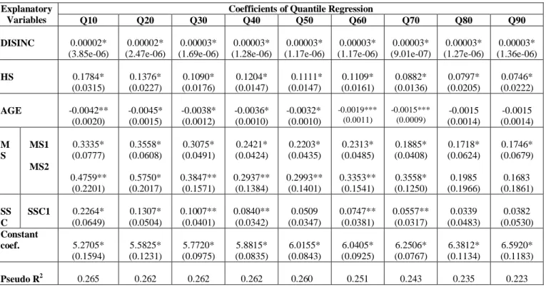
The quantile regression results for rural areas are given in the Table 4. As it can be seen from the table, age, income, marital status, insurance and the size of the household are found significantly. The number of the significant factors affecting the consumption expenditures for rural areas is rather low.

In the rural area, the effect of income on consumption is relatively stable across all consumption expenditures quantiles (approximately 0.003 percent). According to OECD equivalence scale, the size of household raises the consumption expenditures at all quantiles. We can see that the coefficient of size of household at the 10th quantile is 17 percent while the variable at the 90th quantile is about 7 percent. While the consumption expenditures of a single household head are higher than the consumption expenditures of widowed and divorced household head, the consumption expenditures of a married household head are also higher at the 10th, 50th and 90th quantiles. The consumption expenditures of the people registered to the social insurance institution are found higher than the ones of the people not registered at all quantiles. Its effects on the consumption expenditures show a decrease towards upper quantiles (approximately from 25 to 3.7 percent). But it is found insignificant at the 80th and 90th quantiles. Like this variable, MS2 and age variables are also found insignificant at the same quantiles.

Table 4. Results of Quantile Regressions for Rural

(i) *,**,*** indicate significance at the level 1%, 5% and 10%, respectively (ii) Numbers in parentheses are standard errors.

(iii) numbers of observations=1777

6. Conclusion

The analysis of household consumption expenditures, especially of consumer behaviors, enables the following of both social and demographic factors along with the changes in the cultural structure, and development of policies as a result of these impressions. For this reason, it has a significant and vast place in the literature. Although there are many studies examining the consumption expenditures on different goods, there not many studies dealing with the factors affecting total consumption expenditures for the examined country. This study aims to determine the factors affecting the total consumption expenditures. The household consumption expenditures data gathered from Turkish Statistical Institute (TurkStat) in 2009 is used in this study. The models are estimated through the use of all the data, and also the models are estimated separately for urban and rural areas in this study. The estimates are made with quantile regression in order to observe the response of consumption expenditures against the change in the factors dealt at different points.

Explanatory Variables

Coefficients of Quantile Regression

Q10 Q20 Q30 Q40 Q50 Q60 Q70 Q80 Q90 DISINC 0.00002* (3.85e-06) 0.00002* (2.47e-06) 0.00003* (1.69e-06) 0.00003* (1.28e-06) 0.00003* (1.17e-06) 0.00003* (1.17e-06) 0.00003* (9.01e-07) 0.00003* (1.27e-06) 0.00003* (1.36e-06) HS 0.1784* (0.0315) 0.1376* (0.0227) 0.1090* (0.0176) 0.1204* (0.0147) 0.1111* (0.0147) 0.1109* (0.0161) 0.0882* (0.0136) 0.0797* (0.0205) 0.0746* (0.0222) AGE -0.0042** (0.0020) -0.0045* (0.0015) -0.0038* (0.0012) -0.0036* (0.0010) -0.0032* (0.0010) -0.0019*** (0.0011) -0.0015*** (0.0009) -0.0015 (0.0014) -0.0015 (0.0014) M S MS1 MS2 0.3335* (0.0777) 0.4759** (0.2201) 0.3558* (0.0608) 0.5750* (0.2017) 0.3075* (0.0491) 0.3847** (0.1571) 0.2421* (0.0424) 0.2937** (0.1384) 0.2203* (0.0435) 0.2993** (0.1401) 0.2313* (0.0485) 0.3353** (0.1541) 0.1885* (0.0408) 0.3558* (0.1250) 0.1718* (0.0624) 0.1985 (0.1966) 0.1746* (0.0679) 0.1683 (0.1861) SS C SSC1 0.2264* (0.0649) 0.1307* (0.0504) 0.1007** (0.0401) 0.0840** (0.0342) 0.0509 (0.0347) 0.0747** (0.0381) 0.0557** (0.0317) 0.0339 (0.0483) 0.0382 (0.0530) Constant coef. 5.2705* (0.1594) 5.5825* (0.1231) 5.7720* (0.0975) 5.8815* (0.0835) 6.0155* (0.0843) 6.0405* (0.0925) 6.2506* (0.0767) 6.3812* (0.1134) 6.5920* (0.1183) Pseudo R2 0.265 0.262 0.262 0.262 0.260 0.251 0.243 0.235 0.223

When the results of the estimates through the use of all data are examined, it is observed that the expenditures rise as the income increases. This increase is higher especially at upper quantiles. While the consumption expenditures of the urban residents are nearly twice higher than the ones of rural residents at lower quantiles, this overplus decreases at upper quantiles. The expensive and hard living conditions in the urban areas may be a reason for this. The consumption expenditure differences between the rural and urban residents lessen at upper quantiles. The importance of insurance status diminishes at upper quantiles. The type of the household; the consumption expenditures of immediate and extended families are higher than the households composed of a single adult at lower quantiles. The increase in the age raises the consumption expenditures. The ownership status has influence on consumption expenditures at upper quantiles. When the gender variable is examined, it is observed that the consumption expenditures of men are lower than the consumption expenditures of women. When the literature is examined, this result comes as a surprise.

When the models are estimated separately for rural and urban areas, it is possible to see the differences in the factors affecting consumption expenditures. In the estimates through all observations regardless of rural-urban distinction, the lower value of consumption expenditures of men than the consumption expenditures of women are rather close to the values obtained for the same variables in the urban estimates. This result shows that rural areas do not have much influence on the estimation of these variables. The results obtained from the urban estimations are close to the results estimated through the use of all data.

While the age increases the consumption expenditures in general and urban estimations, it decreases the consumption expenditures in the rural estimations. While the variables used in the general estimations are obtained significantly in the urban estimations, same variables do not give significant results in the rural estimations. Only age, income, marital status, insurance, and the size of the household are obtained significantly in the rural estimations. When the results of all the estimated models are examined, especially insurance status is interesting. Insurance variable defines whether the treatment expenses of household are covered in total or in part by any institutions. If the health expenses of individuals are covered by the Social Security Institution, to which s/he registered, the dependant individuals are considered within the scope of compulsory insurance. Thus, being insured is considered as a life guarantee and draws attention as a factor affecting consumption expenditures. The observance of regional differences in consumption expenditures by distinguishing rural and urban areas, and the determination of the factors affecting total consumption expenditures for a country through the use of all data may be informative for policy-makers.

References

Blundell, R., &Walker, I. A. (1985). Household production specification of demographic variables in demand analysis. The Economic Journal, 94, 59-68.

Brown, J.A.C. (1954). The consumption of food in relation to household composition and ıncome. Econometrica, 22, 444-460.

Burney, N.A.., & Akmal, M. (1991). Food demand in pakýstan: an application of the extended linear expenditure system. Journal of Agricultural Economics, 42, 185-195.

Chatterjee, S., & Michelini, C. (1998). Household consumption equivalence scales: some estimates fromnew zealand household expenditure and ıncome survey data. Australian & New Zealand Journal Statistic, 40, 141-150.

Gustafsson, B., & Li, S. (2002). Income inequality within and across counties in rural China 1988 and 1995. Journal of Development Economics, 69, 179–204.

Halvorsen, R.,& Palmquist, R.(1980). The Interpretation of dummy variables in semilogarithmic equations. American Economic Review, 70, 474-475.

Kennedy, P. (1981). Estimation with correctly interpreted dummy variables in semilogarithmic equations. American Economic Review, 71, 801.

Koenker, R.,& Bassett, G.(1978). Regressions quantiles. Econometrica, 46, 33 – 50.

Koenker, R., & Bassett, G. (1982). Robust tests for heteroscedasticity based on regression quantiles. Econometrica, 50, 43-62.