C om mun.Fac.Sci.U niv.A nk.Series A 1 Volum e 66, N umb er 2, Pages 297–310 (2017) D O I: 10.1501/C om mua1_ 0000000820 ISSN 1303–5991
http://com munications.science.ankara.edu.tr/index.php?series= A 1
STATISTICAL INFERENCE FOR THE BURR TYPE III DISTRIBUTION UNDER TYPE II CENSORED DATA
Ö. ALTINDA ¼G, M. N. ÇANKAYA, A. YALÇINKAYA, AND H. AYDO ¼GDU
Abstract. In this study, estimation and prediction problems for the Burr type III distribution under type II censored data are considered. Maximum likeli-hood and maximum product spacing estimation methods are used to estimate model parameters. EM algorithm is employed to obtain maximum likelihood estimates. Unobserved future order statistics are predicted with best unbiased prediction method. A simulation study is carried out to exhibit performance of the estimation methods. Further, a numerical example is presented to illus-trate the usefulness of the Burr III distribution.
Keywords: Burr III distribution, type II censoring, maximum likelihood, EM algorithm, maximum product spacing, inference
1. Introduction
Irwing W. Burr [1] introduced a distribution family which includes twelve distri-bution types. Among these distridistri-butions, Burr type III (BIII) and type XII (BXII) have attracted considerable attention in the literature. It should be noted that they are reciprocal. Lindsay [2] used BIII distribution to model diameter distributions of forest stands as an alternative to Weibull distribution. Shao [3] has modelled the NOEC toxicity data with BIII distribution. Zimav et al. [4] showed that BXII distribution is a useful model for failure data in reliability studies. Some other usages of the BIII and BXII distributions can be found in [5-10]. However, BIII distribution is more ‡exible to …t data than BXII in the sense that it provides wider skewness and kurtosis region. One can refer to Rodriguez [11] and Tadikamalla [12] for the details.
When investigating lifetime characteristics of a unit, it is aimed to …t failure data with a ‡exible distribution. Since BIII distribution can properly approximates many classical lifetime models such as Weibull, gamma and lognormal [13], it is
Received by the editors: December 25, 2016; Accepted: February 10, 2017. 2010 Mathematics Subject Classi…cation. Primary 62F10, 62N01, 62N02.
Key words and phrases. Burr III distribution, type II censoring, maximum likelihood, EM algorithm, maximum product spacing, inference.
c 2 0 1 7 A n ka ra U n ive rsity C o m m u n ic a tio n s d e la Fa c u lté d e s S c ie n c e s d e l’U n ive rs ité d ’A n ka ra . S é rie s A 1 . M a th e m a t ic s a n d S t a tis tic s .
worthwhile to model failure data with BIII distribution. So, BIII distribution plays an important role in lifetime analysis. In survival and reliability context, some censoring schemes are applied due to time and cost restrictions. A commonly used censoring scheme is type II censoring in which only the …rst r n failures among the n units are observed. Wingo [14] studied the maximum likelihood estimation for BXII distribution under type II censoring. Wang and Cheng [15] and Sayyareh [16] derived the expectation-maximization (EM) procedure for BXII distribution under multiple censoring and type II censoring, respectively. It should be pointed out that once the parameters of BXII distribution have been estimated from a random sample, the parameters of BIII distribution have already been obtained because of their reciprocal property, vice versa. However, this relation does not hold for the type II censored data though it holds for the complete sample. This fact can be explained as follows.
Let the random variable Y has BXII distribution, then X = 1=Y has BIII dis-tribution. So, when a complete sample from BIII distribution is observed, the estimates of parameters can be obtained from the estimation procedure of BXII model by replacement of each observation with its reciprocal. Let type II censored sample from BIII distribution has been observed. It is clear that, the inverses of these observations do not correspond to the type II censored sample from BXII dis-tribution. Thus, estimation procedure for the parameters of BIII distribution under type II censoring has to be derived. Moradi et al. [17] have considered so called exponentiated-BIII distribution under type II censored data. However, extending the BIII distribution with exponentiation is meaningless since the distribution they have derived corresponds to reparametrized version of the BIII distribution. Azizi et al. [18] and Singh et al. [19] have studied parameter estimation for the BIII distribution under type II hybrid censoring and type II progressive censoring, re-spectively. It should be noted that these are generalizations of the classic type II censoring. In this study, estimation problem for the parameters of BIII distribution and prediction of the unobserved future order statistics under type II censored data are considered. Unlike the previous studies, the maximum product spacing (MPS) method is also taken into account as an alternative.
Remainder of the article is organized as the following. In Section 2, ML and MPS estimation methods for the parameters are considered. The EM algorithm is used to obtain ML estimates. Asymptotic variances and covariance of the ML estimates are calculated with missing information principle (MIP) introduced by Louis [20]. The Section 3 is divided to the prediction of unobserved future order statistics for the type II censored sample. A comprehensive simulation study is carried out to evaluate the performances of ML and MPS estimation methods with di¤erent parameter, sample size and censoring settings in Section 4. An illustrative real data example is studied in Section 5. Finally, the study is concluded in Section 6.
2. Parameter Estimation
The cumulative distribution function (cdf) and the probability density function (pdf) of the BIII distribution are given by
F (x; c; k) = 1 + x c k; x 0; c; k > 0; (2.1) f (x; c; k) = kcx (c+1) 1 + x c (k+1); x 0; c; k > 0; (2.2) respectively. The parameters c and k are the shape parameters of the distribu-tion. Suppose that X1; X2; :::; Xn be independent and identically BIII distributed
random variables representing the lifetimes of n independent units. For type II censoring case, only the …rst pre…xed r (r n) failures, say X1:n; X2:n; :::; Xr:n,
are observed. These failures correspond to the …rst r order statistics of the random sample X1; X2; :::; Xn. To estimate the parameters of the BIII distribution we will
consider ML and MPS methods, respectively.
2.1. ML method. The likelihood function of the BIII distribution under type II censored data is given by
L (c; k; x) = n! (n r)! r Y i=1 f (xi:n; c; k) [1 F (xr:n; c; k)]n r = n! (n r)!k rcrh1 1 + x c r:n kin rYr i=1 xi:n(c+1) 1 + xi:nc (k+1) (2.3) where x = (x1:n; x2:n; :::; xr:n). It is generally tractable to work with log-likelihood
function instead of the likelihood function. Therefore, the log-likelihood function is log L (c; k; x) = constant + r (log c + log k) + (n r) log 1 1 + xr:nc k
(c + 1) r X i=1 log (xi:n) (k + 1) r X i=1 log 1 + xi:nc : (2.4) The ML estimates of c and k are the arguments maximizing the log L function. For the Equation (2.4), the ML estimators cannot be obtained in an analytical form. One way to obtain ML estimates of c and k is that the …rst partial derivatives of the log L function with respect to c and k are equated to zero and these nonlinear equations are solved by a numerical procedure such as Newton-Raphson (NR). However, when employing the NR method some errors such as non-convergence or convergence to wrong value can occur. This may result in incorrect estimates. Dempster et al. [21] developed a method called EM to calculate the ML estimates in the presence of missing data. The EM algorithm is based on repeating the E and M steps until convergence occurs. Since the log-likelihood function increases in each repetition, the EM algorithm provides remarkable results for computation of the ML estimates. For the type II censoring case, the censored observations can
be thought of missing data and therefore the EM algorithm can be used to obtain the ML estimators. For the type II censored data with given pre…xed constant r, let us denote the observed and censored data by X = (X1:n; X2:n; :::; Xr:n) and
Z = (Z1; Z2; :::; Zn r), respectively. Then the complete data is W = (X; Z).
The log-likelihood function for the complete sample W is expressed as log Lc(c; k; W ) = n (log k + log c) (c + 1)
n X i=1 log wi (k + 1) n X i=1 log(1 + wi c) = n (log k + log c) (c + 1) r X i=1 log xi:n+ n r X i=1 log Zi ! (k + 1) r X i=1 log 1 + xi:nc + n rX i=1 log 1 + Zi c ! (2.5) In the E step of the algorithm, the conditional expectation of the log Lc given
X1:n = x1:n; :::; Xr:n = xr:n, that is EZjX[log Lc(c; k; W )] has to be calculated.
By the theorem of Ng et al. [22], given X = (x1:n; :::; xr:n), the unobserved variables
Z1; Z2; :::; Zn r are conditionally independent and their conditional distributions
are identical truncated BIII distribution with left truncation at xr:n. Therefore,
EZjX [log Lc(c; k; W )] = n (log k + log c) (c + 1) r X i=1 log xi:n+ n r X i=1 E [log ZijZi> xr:n] ! (k + 1) r X i=1 log 1 + xi:nc + n rX i=1 E log 1 + Zi c jZi> xr:n ! ; (2.6) where E log 1 + Zi c jZi > xr:n = ck 1 F (xr:n) Z 1 xr:n log 1 + z c z (c+1) 1 + z c (k+1)dz = 1 k (1 + xr:nc) k 1 1 + xr:nc k log 1 + x c r:n ; (2.7) E [log ZijZi> xr:n] = ck 1 F (xr:n) Z 1 xr:n (log z) z (c+1) 1 + z c (k+1)dz: (2.8) The details for the integration are given in the appendix.
In the M step of the algorithm, the function EZjX[log Lc(c; k; W )] is
max-imized with respect to the parameters c and k. Let us write (c; k; xr:n) =
ML estimates ^c and ^k of the parameters c and k are obtained by repeating the iteration c(h+1); k(h+1) = arg max c;k>0 n (log k + log c) (c + 1) " r X i=1 log xi:n+ (n r) c(h); k(h); xr:n # (k + 1) " r X i=1 log 1 + xi:nc + (n r) c(h); k(h); xr:n #) ; h = 0; 1; 2; :::;
until (c(h+1) c(h); k(h+1) k(h)) < is satis…ed, where k:k stands for the
Euclidean norm in R2, c
(0) and k(0) are the initial guesses of ^c and ^k and > 0
denotes pre-speci…ed tolerance level. Thus, ^c = c(h+1) and ^k = k(h+1) for which h
is the smallest integer such that the convergence criterion holds.
The maximization procedure can be done as given by Kundu and Pradhan [23]. First, c(h+1) is obtained by solving the …xed point type equation
g (c) = c; where g (c) = n " r X i=1 log xi:n+ (n r) c(h); k(h); xr:n (k (c) + 1) r X i=1
xi:nclog xi:n
1 + xi:nc # 1 (2.9) and k (c) = n " r X i=1 log 1 + xi:nc + (n r) c(h); k(h); xr:n # 1 : (2.10) Then k(h+1) is obtained as k(h+1)= k c(h+1) .
One of the advantages using the EM algorithm when computing the ML estimates is that it enables us to obtain Fisher information matrix easily via MIP. The MIP is based on the idea
Observed information = Complete information - Missing information. Let us write = (c; k) : Then, the complete information and the missing infor-mation matrices are de…ned as
Icom( ) = nE " @2log f (X; ) @c2 @2log f (X; ) @c@k @2log f (X; ) @c@k @2log f (X; ) @k2 # ; (2.11) Imis( ) = (n r) E " @2log f (X jX>xr:n; ) @c2 @2log f (X jX>xr:n; ) @c@k @2log f (X jX>xr:n; ) @c@k @2log f (X jX>xr:n; ) @k2 # ; (2.12)
respectively, where X is BIII random variate and f is the pdf of X. Thus, the observed information matrix is given as
Iobs( ) = Icom( ) Imis( ) : (2.13)
The elements of these matrices are given in the appendix. By inverting the ma-trix Iobs( ), one can obtain the asymptotic variance-covariance matrix of the ML
estimates ^c and ^k.
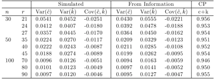
In order to evaluate the performance of approximation for the variances and covariance of the ML estimates obtained from the information matrix, we have carried out a Monte Carlo simulation with 1000 replications. For the sake of simplicity, we take c = 1 and k = 1. The variances and covariance obtained from simulation and information matrix are given in Table 1. We also give cov-erage probability (CP) of %95 con…dence interval of ^c + ^k. It is ratio satisfying c + k 2 (^c + ^k 1:96
q
Var(^c + ^k); ^c + ^k + 1:96 q
Var(^c + ^k)). Here, Var(^c + ^k) = Var(^c) + Var(^k) + 2Cov(^c + ^k) and it is computed from information.
Table 1. Variances, covariance and coverage probability of ML estimates using the EM algorithm
Simulated From Information CP n r Var(^c) Var(^k) Cov(^c; ^k) Var(^c) Var(^k) Cov(^c; ^k) c+k 30 21 0.0541 0.0452 -0.0251 0.0430 0.0555 -0.0221 0.956 24 0.0412 0.0407 -0.0180 0.0392 0.0478 -0.0188 0.953 27 0.0357 0.0445 -0.0170 0.0364 0.0450 -0.0162 0.954 50 35 0.0224 0.0270 -0.0117 0.0209 0.0329 -0.0123 0.951 40 0.0222 0.0243 -0.0087 0.0211 0.0285 -0.0108 0.952 45 0.0188 0.0274 -0.0089 0.0199 0.0262 -0.0095 0.954 100 70 0.0096 0.0126 -0.0051 0.0094 0.0163 -0.0059 0.946 80 0.0101 0.0123 -0.0049 0.0097 0.0141 -0.0052 0.950 90 0.0097 0.0120 -0.0046 0.0095 0.0127 -0.0047 0.955
It is seen from the Table 1 that the approximations for the variances and co-variance determined from the information matrix are satisfactory in the case of moderate n and low censoring. The approximations become more accurate as n increases even if the censoring level is high. Also, the values of CP are near 0:95 in almost all cases.
2.2. MPS method. The MPS method was introduced as an alternative to ML method by Cheng and Amin [24] and independently by Ranneby [25]. Their aim is to overcome an unboundedness problem of the likelihood with a pdf having shifted origin for which the ML estimators may become inconsistent. For comprehensive content, one can refer to Ekström [26]. MPS and ML estimators are asymptotically equal and have same asymptotic su¢ ciency, consistency and e¢ ciency properties as pointed out in Cheng and Amin [24]. The MPS method is based on maximizing the product of consecutive di¤erences between values of the cdf at ordered observations.
Considering the probability integral transform, it is clear that MPS method chooses the values as estimates which make the spacings as uniform as possible. Since the cdf is being used as base function, there does not occur any unboundedness problem. The MPS estimators of c and k are given for complete and type II censored data as follows. Let X = (X1; X2; :::; Xn) be a complete sample from BIII distribution.
Therefore, the MPS estimates are the arguments maximizing the function G(c; k; x) G (c; k; x) =
n+1Y i=1
[F (xi:n; c; k) F (xi 1:n; c; k)] ; (2.14)
with respect to c and k where (x1:n; x2:n; :::; xn:n) is the ordered sample and
F (x0:n; c; k) := 0, F (xn+1:n; c; k) := 1. For the type II censored sample, the
function G (c; k; x) can be obtained similarly as given in Ng et al. [27] by G (c; k; x) =
r+1Y i=1
[F (xi:n; c; k) F (xi 1:n; c; k)] [1 F (xr:n; c; k)]n r; (2.15)
where x = (x1:n; x2:n; :::; xr:n) and F (xr+1:n; c; k) is taken to be 1 for convenience.
Hence, the MPS estimators are ~
c; ~k = arg max
c;k>0G (c; k; X) : (2.16)
Since there are no analytic expressions for ~c and ~k, they can be obtained by nu-merical non-linear optimization techniques.
3. Prediction of future order statistics
In this section, we will consider predicting the unobserved future order statistics for type II censored data. As well as, there are some methods, we prefer to use the best unbiased prediction method. Let X = (X1:n; X2:n; :::; Xr:n) be the sample
will being observed and Yk= Xr+k:n, k = 1; :::; n r be the unobservable variables
for the type II censored data. Therefore, the best unbiased predictor (BUP) for Yk,
k = 1; :::; n r is de…ned as ^
Yk = E [YkjX] : (3.1)
Considering the Markovian property of order statistics, E [YkjX] = E [YkjXr:n] :
It should be noted that, Yk, k = 1; :::; n r, corresponds to the kth order statistic
of n r units from the truncated BIII distribution with left truncation at xr:n,
given Xr:n= xr:n. Therefore, given Xr:n= xr:n, the pdf of Yk is
fk(yjxr:n; c; k) = k n r k [F (y; c; k) F (xr:n; c; k)] k 1 [1 F (y; c; k)]n r k [1 F (xr:n; c; k)]r n; y > xr:n; (3.2)
where f and F are the pdf and cdf of BIII distribution with parameters c and k, respectively. Thus, the BUP for Yk, k = 1; :::; n r is
^ Yk=
Z 1
xr:n
yfk(yjxr:n; ^c; ^k)dy; (3.3)
where ^c and ^k are the ML estimates based on (x1:n; x2:n; :::; xr:n).
4. Simulation study
In this section, we will carry out a Monte Carlo simulation in order to investigate how the ML and MPS estimation methods perform for BIII distribution under di¤erent settings for sample sizes, censoring and parameter values. For this purpose, the number of replications is chosen as N = 104. Sample sizes are taken as 20, 40, 60 and 100. Two censoring levels, %10 and %30, are considered for each sample sizes. It should be noted that the pdf of the BIII distribution is L-shaped when ck 1 and unimodal when ck > 1. So, we both consider L-shaped and unimodal cases by choosing the parameters as (c = 1; k = 1), (c = 0:6; k = 0:8), (c = 2; k = 0:4) and (c = 1; k = 2), (c = 0:8; k = 1:5), respectively. For convergence criteria of the EM algorithm, we take the tolerance level as = 10 5. All the simulations are conducted in MATLABT M program. The nonlinear optimization tools are used for
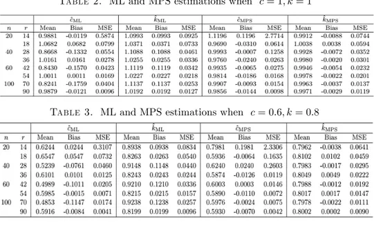
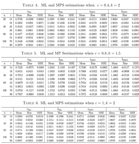
computation of the MPS estimators. We present the simulation mean, bias and mean square error (MSE) values for both ML and MPS estimators of c and k in Tables 2-6.
Table 2. ML and MPS estimations when c = 1; k = 1
Table 4. ML and MPS estimations when c = 0:4; k = 2
Table 5. ML and MP Sestimations when c = 0:8; k = 1:5
Table 6. ML and MPS estimations when c = 1; k = 2
The simulation results have been summarized as follows. First of all, the be-haviors of the ML and MPS estimators do not show a discrepancy depending on whether the pdf is L-shaped or unimodal. The biases of ^c and ^k are a bit greater, compared to the biases of ~c and ~k. Although the biases of ~c and ~k do not change depending on the censoring proportion, the biases of ^c and ^k increase as the censor-ing proportion increases. All the biases get smaller as the sample size gets larger. ~
k mostly underestimate the parameter k for all cases whereas ^k overestimates ab-solutely. Similarly, ~c usually underestimates the parameter c. However, there is no such a case for ^c. For each sample size, the MSE values of all the estimators increase when the censoring proportion gets larger. Also, all the MSE values get smaller as the sample size increases. Since the ML and MPS estimators are consistent, this
is an expected situation. Further, it is observed that there is not any remarkable superiority between the ML and MPS estimators with respect to the MSE criterion, that is, all the MSE values are close to each other for both methods in much cases.
5. Illustrative example
In this section, we will consider a real data set given by Mann and Fertig [28]. This data set is also studied by Prakash and Singh [29] from a Bayesian perspective. The data set contains 10 failure times of airplane components of total 13 items. The censoring scheme is type II censoring with r = 10 and n = 13. The data set is
f0:22; 0:50; 0:88; 1:00; 1:32; 1:33; 1:54; 1:76; 2:50; 3:00g :
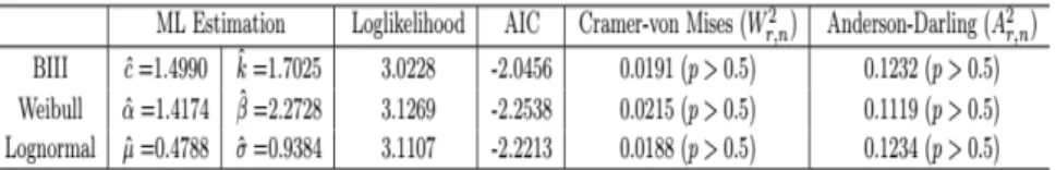
If we model this data set with BIII distribution, the ML estimates of parameters and the related standard errors (in parenthesis) are obtained as ^c = 1:4990(0:1458) and ^k = 1:7025(0:2279). This data set was also studied in Crowder et al. [30]. They considered Weibull and lognormal models. For these models, the rough estimates were found by graphical technique as ^ = 1:4; ^ = 2:2; ^ = 0:5; ^ = 1.
Here, and are shape and scale parameters of the Weibull distribution, re-spectively, and are the parameters of lognormal distribution which are mean and standard deviation of the corresponding normal distribution, respectively. We have computed the ML estimations of these parameters as given in Table 7. In order to compare BIII, Weibull and lognormal models for this data set, we consider loglikelihood, Akaike information criteria (AIC) values and Cramér-von Mises and Anderson-Darling test statistics. The results are presented in Table 7. It should be noted that the Cramér-von Mises and Anderson-Darling test statistics for the type II censored data are computed by using the W2
r;n and A2r;n statistics given
in D’Agostino and Stephens [31] at p. 114. Critical points of the W2
r;n and A2r;n
statistics at signi…cance level 0:5 are nearly 0:085 and 0:503, respectively as given in Table 4.5 of [31]. So, the associated p-values of both statistics for BIII, Weibull and lognormal models are much bigger than 0.5.
Table 7. Comparison of BIII, Weibulland Lognormal models
From Table 7, it can be considered that the BIII is successful to model this data set as much as Weibull and lognormal models. This indicates that the BIII distribution may be a good alternative for …tting lifetime data sets. Furthermore, the predictions for the unobserved variables are computed as ^Y1 = 4:0601, ^Y2 =
6:3858 and ^Y3 = 20:0207 via BUP approach. When a sample of size 13 from BIII
three observations of ordered sample are computed averagely as 4:2975, 6:8485 and 19:9901. These values agree with the predictions, as expected.
6. Conclusion
In this study, we have concerned with the statistical inference problem for the BIII distribution under type II censored data. For this purpose, we have taken into account the ML and MPS methods. We have implemented the EM algorithm for the computation of the ML estimators. Also, the information matrix is derived by means of MIP. The unobserved future order statistics have been predicted via BUP approach. Monte Carlo simulations indicate that in order to estimate the model parameters, both of the ML and MPS methods can be used. Especially, if the censoring proportion is large we suggest to use the MPS method since absolute biases of the MPS estimators are lower than that of ML estimators. Finally, the real life examination has illustrated modeling capacity of the BIII distribution.
Acknowledgement
The authors would like to express their gratitude to an anonymous referee for the valuable comments and suggestions.
7. Appendix
The integral given in Equation (2.7) is analytically obtained by …rst applying 1 + z c= y transformation and then applying partial integration. These steps are
as follows: E log 1 + Zi c jZi > xr:n = ck 1 F (xr:n) Z 1 xr:n log 1 + z c z (c+1) 1 + z c (k+1)dz = k 1 F (xr:n) Z 1+x c r:n 1 log (y)y (k+1)dy = k 1 F (xr:n) " log (y) y k k j 1+xr:nc 1 + Z 1+x c r:n 1 y (k+1)dy # = k 1 F (xr:n) " log 1 + x c r:n (1 + x c r:n) k k ! + 1 k2(1 F (xr:n)) # = 1 k (1 + xr:nc) k 1 1 + xr:nc k log 1 + xr:nc :
Existence of the expectation given in Equation (2.8) can be easily shown by simple calculus.
To get the complete information Icom( ) the second partial derivatives of log f
with respect to c and k are @2log f @c2 = 1 c2 (k + 1) log2(x)x c (1 + x c)2; @2log f @k2 = 1 k2; @2log f @c@k = log (x)x c 1 + x c :
Therefore the elements of the complete information based on n units are Icom( )11= n 1 c2 + (k + 1) E " log2(X)X c (1 + X c)2 #! ; Icom( )12= nE log (X)X c 1 + X c ; Icom( )21= Icom( )12; Icom( )22= n k2;
where X is BIII random variable. Since the expectations Ehlog2(X)X c
(1+X c)2 i and E h log (X)X c 1+X c i
cannot be obtained analytically, they have to be computed numer-ically. The missing information is obtained in a similar manner. Skipping the derivation steps, we obtain the elements of the missing information as
Imis( )11= (n r) 1 c2 + (k + 1) E " log2(X)X c (1 + X c)2 jX > xr:n # + A ! ; Imis( )12= (n r) E log (X)X c 1 + X c jX > xr:n + B ; Imis( )21= Imis( )12; Imis( )22= (n r) 1 k2 C ; where A = log2(xr:n)k h (1 + x c r:n) k (xc r:n k) xcr:n i (1 + xc r:n) 2 1 1 + xr:nc k 2 ; B =(1 + x c r:n) k 1 log(xr:n)xr:nc 1 1 + xr:nc k 1 k log 1 + x c r:n 1 1 + xr:nc k 1 ;
C =log 2 (1 + x c r:n)(1 + xr:nc) k 1 1 + xr:nc k 2 :
Here, the expectations have to be computed numerically since they have no ana-lytical solution. Also, it should be pointed out that all the expectations related with the information matrices exist. It is straightforward from the existence of E[log(X)].
References
[1] Burr, I. W. (1942). Cumulative frequency functions. The Annals of mathematical statistics 13(2): 215-232.
[2] Lindsay, S. R., et al. (1996). Modelling the diameter distribution of forest stands using the Burr distribution. Journal of Applied Statistics 23(6): 609-619.
[3] Shao, Q. (2000). Estimation for hazardous concentrations based on NOEC toxicity data: an alternative approach. Environmetrics 11(5): 583-595.
[4] Zimmer, W. J., et al. (1998). The Burr XII distribution in reliability analysis. Journal of Quality Technology 30(4): 386.
[5] AbdelGhaly, A. A., et al. (1997). The use of Burr type XII distribution on software reliability growth modelling. Microelectronics and Reliability 37(2): 305-313.
[6] Shankar, G. and Sahani, V. (1994). The Study of a Maintenance Float Model with Burr Failure Distribution. Microelectronics and Reliability 34(9): 1513-1517.
[7] Liu, P. H. and Chen, F. L. (2006). Process capability analysis of non-normal process data using the Burr XII distribution. International Journal of Advanced Manufacturing Technology 27(9-10): 975-984.
[8] Gove, J. H., et al. (2008). Rotated sigmoid structures in managed uneven-aged northern hardwood stands: a look at the Burr Type III distribution. Forestry 81(2): 161-176. [9] Kar, R., et al. (2010). A closed form Delay Evaluation Approach using Burr’s Distribution
Function for High Speed On-Chip RC Interconnects. 2010 Ieee 2nd International Advance Computing Conference : 129-133.
[10] Ganora, D. and Laio, F. (2015). Hydrological Applications of the Burr Distribution: Practical Method for Parameter Estimation. Journal of Hydrologic Engineering 20(11).
[11] Rodriguez, R. N. (1977). A guide to the Burr type XII distributions. Biometrika 64(1): 129-134.
[12] Tadikamalla, P. R. (1980). A look at the Burr and related distributions. International Sta-tistical Review/Revue Internationale de Statistique : 337-344.
[13] Zoraghi, N., et al. (2012). Estimating the four parameters of the Burr III distribution using a hybrid method of variable neighborhood search and iterated local search algorithms. Applied Mathematics and Computation 218(19): 9664-9675.
[14] Wingo, D. R. (1993). Maximum likelihood estimation of Burr XII distribution parameters under type II censoring. Microelectronics Reliability 33(9): 1251-1257.
[15] Wang, F.K. and Cheng, Y. (2010). EM algorithm for estimating the Burr XII parameters with multiple censored data. Quality and Reliability Engineering International 26(6): 615-630. [16] Panahi, H. and Sayyareh, A. (2014). Parameter estimation and prediction of order statistics
for the Burr Type XII distribution with Type II censoring. Journal of Applied Statistics 41(1): 215-232.
[17] Moradi, N., et al. (2014). Estimation of the parameters of a exponentiated Burr type III distribution under type II censoring. Journal of Statistical Sciences 8(1): 93-109.
[18] Azizi, A. Z., et al. (2013). Inference about the Burr type III distribution under type-II hybrid censored data. Journal of Statistical Research of Iran 10(2): 209-233.
[19] Singh, D. P., et al. (2016). Estimation and prediction for a Burr III distribution with progres-sive censoring. Communication in Statistics - Theory and Methods. Accepted manuscript. DOI:10.1080/03610926.2016.1213290.
[20] Louis, T. A. (1982). Finding the observed information matrix when using the EM algorithm. Journal of the Royal Statistical Society. Series B (Methodological): 226-233.
[21] Dempster, A. P., et al. (1977). Maximum likelihood from incomplete data via the EM algo-rithm. Journal of the Royal Statistical Society. Series B (Methodological): 1-38.
[22] Ng, H., et al. (2002). Estimation of parameters from progressively censored data using EM algorithm. Computational Statistics & Data Analysis 39(4): 371-386.
[23] Kundu, D. and Pradhan, B. (2009). Estimating the parameters of the generalized exponential distribution in presence of hybrid censoring. Communications in Statistics - Theory and Methods 38(12): 2030-2041.
[24] Cheng, R. and Amin, N. (1983). Estimating parameters in continuous univariate distributions with a shifted origin. Journal of the Royal Statistical Society. Series B (Methodological): 394-403.
[25] Ranneby, B. (1984). The maximum spacing method. An estimation method related to the maximum likelihood method. Scandinavian Journal of Statistics : 93-112.
[26] Ekström, M. (2008). Alternatives to maximum likelihood estimation based on spacings and the Kullback–Leibler divergence. Journal of Statistical Planning and Inference 138(6): 1778-1791.
[27] Ng, H., et al. (2012). Parameter estimation of three-parameter Weibull distribution based on progressively Type-II censored samples. Journal of Statistical Computation and Simulation 82(11): 1661-1678.
[28] Mann, N. R. and Fertig, K. W. (1973). Tables for obtaining Weibull con…dence bounds and tolerance bounds based on best linear invariant estimates of parameters of the extreme-value distribution. Technometrics 15(1): 87-101.
[29] Prakash, G. and Singh, D. (2009). A Bayesian shrinkage approach in Weibull type-II censored data using prior point information. REVSTAT–Statistical Journal 7(2): 171-187.
[30] Crowder, M.J., et al. (1991). Statistical Analysis of Reliability Data. Great Britain: Chap-mann&Hall.
[31] D’agostino, R.B. and Stephens, M.A. (1986). Goodness of Fit Techniques. New York: Marcel Dekker.
Current address : Ömer Alt¬nda¼g: Bilecik ¸Seyh Edebali University, Faculty of Arts and Science, Department of Statistics, Bilecik, Turkey.
E-mail address : [email protected], [email protected]
Current address : Mehmet Niyazi Çankaya: U¸sak University, Faculty of Arts and Science, Department of Statistics, U¸sak, Turkey.
E-mail address : [email protected], [email protected]
Current address : Abdullah Yalç¬nkaya: Ankara University, Faculty of Science, Department of Statistics, Ankara, Turkey.
E-mail address : [email protected]
Current address : Halil Aydo¼gdu: Ankara University, Faculty of Science, Department of Sta-tistics, Ankara, Turkey.