Oil price, oil price volatility and natural gas

(1)

OIL PRICE, OIL PRICE VOLATILITY

AND NATURAL GAS

A Master’s Thesis

by

MÜRŞİDE RABİA ERDOĞAN

The Department of

Economics

İhsan Doğramacı Bilkent University

Ankara

September 2017

MÜRŞ İD E RAB İA ERDOĞ AN OI L P R ICE, O IL P R ICE V OL AT IL IT Y AN D N AT U R AL GA S B il ke nt Univer sit y 2017

(2)

(3)

(4)

OIL PRICE, OIL PRICE VOLATILITY

AND NATURAL GAS

The Graduate School of Economics and Social Sciences

of

İhsan Doğramacı Bilkent University

By

MÜRŞİDE RABİA ERDOĞAN

In Partial Fulfillment of the Requirements for The Degree of

MASTER of ARTS in Economics

The Department of

Economics

İhsan Doğramacı Bilkent University

Ankara

(5)

(6)

iii

ABSTRACT

OIL PRICE OIL PRICE VOLATILITY AND NATURAL GAS

Erdoğan, Mürşide Rabia M.A., Department of Economics Supervisor: Prof. Dr. Hakan Berument

Co-Supervisor: Dr. Eray Yücel

September 2017

Natural gas market has been developing and transportation and storage methods have

been improving. Due to substitution between natural gas and oil in various sectors such

as power generation, oil price and oil price volatility may reflect these changes in

natural gas markets. We employ four ratios regarding the role natural gas markets.

With these ratios, we successfully show that increase in production of natural gas or

decrease in production of oil cause decline in oil price volatility with in a set of

autoregressive conditional heteroscedasticity models.

Keywords: LNG, Natural Gas Market and Oil Price Volatility

(7)

iv

ÖZET

PETROL FİYATLARI, PETROL FİYATLARININ DEĞİŞKENLİĞİ VE DOĞAL GAZ

Erdoğan , Mürşide Rabia Yüksek Lisans, İktisat Bölümü Tez danışmanı: Prof. Dr. Hakan Berument

2. Tez Danışmanı: Dr. Eray Yücel Eylül 2017

Doğalgaz piyasası günümüzde ulaştırma ve depolama yöntemlerini değiştirilmekte ve gelişmektedir. Çeşitli sektörlerdeki kullanım, doğalgaz ile petrolü ikame mal haline getirmekte, böylece doğal gaz piyasasındaki bu değişimler petrol fiyatı ve petrol fiyatındaki oynaklığa yansıyabilmektedir. Araştırmamızda arz ve talep yapısını gösteren ve doğalgaz ve petrol arasında geçişi yansıttığını düşündüğümüz dört farklı üretim ve tüketim oranı kullandık. Bu incelemeleri yaparken petrol fiyatlarındaki yoğun oynaklıktan dolayı ve doğalgazdaki değişimin koşullu varyans değişkeni üzerindeki etkisini incelemek için ARCH modeli kullandık. Çalışmamızda, doğal gaz üretiminde artış ya da petrol üretiminde azalmanın petrol fiyatındaki oynaklığın azalmasına neden olduğunu tespit ettik.

(8)

v

ACKNOWLEDGEMENTS

First, I would like to thank to my family for their assistance, guidance and support. Especially, I would appreciate my mum for her unending love.

Second, I want to express my deepest thanks and respect to my thesis advisor, effective teacher, Hakan Berument, who teaches the most in the least period of time. Then I would like to thank to Eray Yücel for his support and guidance.

Besides, special thanks to Tarık Kara, Kemal Yıldız, Çağrı Sağlam, Emin Karagözoğlu and Aygün Dalkıran for listening me patiently.

Also thanks to my friends in Bilkent University; Asu İşbilen, Zeynep Yoldaş, Betim Melis Tan, Fatih Öztürk, Ebru Selderesi, Ece Teoman, Oral Ersoy Dokumacı and Berk İdem.

It is always a pleasure to know family of economics department in Bilkent University, because I have learnt from them a lot, not just about economics but also way of life.

(9)

vi

LIST OF TABLES

1.TABLE 1: Correlation Table ... 18

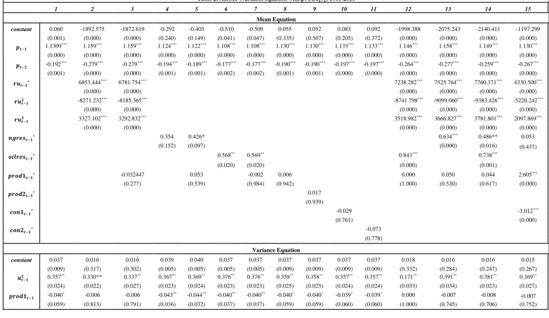
2.TABLE 2:ARCH (variance equation with Prod1) 1988-2016 ... 22

3.TABLE A1: ARCH (variance equation with Prod2) 1988-2016 ... 32

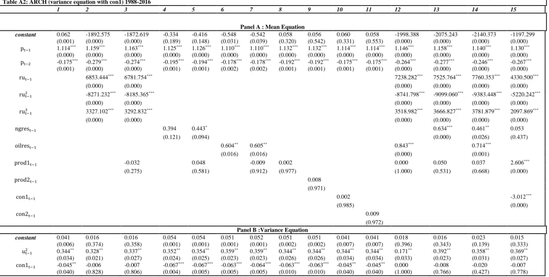
4.TABLE A2:ARCH (variance equation with Con1) 1988-2016 ... 33

5.TABLE A3:ARCH (variance equation with Con2) 1988-2016 ... 34

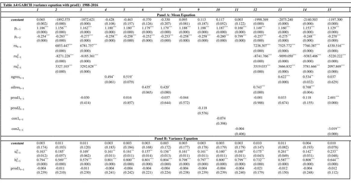
6.TABLE A4:GARCH (variance equation with Prod1) 1988-2016 ... 35

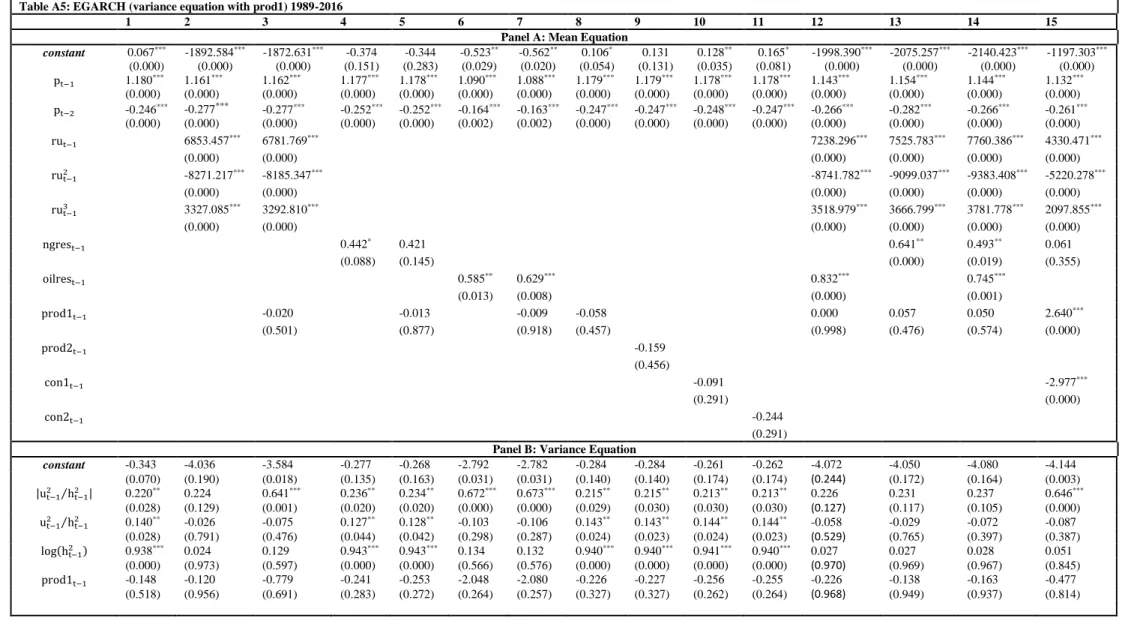
7.TABLE A5:EGARCH (variance equation with Prod1) 1988-2016 ... 36

8.TABLE A6:ARCH (variance equation with Prod1) 1988-1992 ... 37

(11)

viii

LIST OF FIGURES

1.FIGURE 1: Brent Prices ... 12

2.FIGURE 2: Refinery Utilization ... 13

3.FIGURE 3: Growth Of Proven Reserves ... 14

4.FIGURE 4:Consumption Ratios ... 15

(12)

1

CHAPTER 1 INTRODUCTION

Natural gas and oil are substitute products in a degree. This substitution is expected to affect crude oil prices and its volatility. Initially, we will look at the natural gas and oil substitutability with investigation from different perspective. First of all, natural gas has become a crucial source of energy for industrial consumption and power generation, that force to switch from oil to natural gas (U.S. Energy Information Administration, 2016). Thus, lower prices of natural gas contribute competitiveness of energy market due to its growth in demand where natural gas is available. Second, competition in investment decision on energy commodities and supply side of the market. Investment on drilling activity, namely rise in proven reserves of oil and natural gas, is highly related with current and expected prices, thus investments may switch between them relative to energy prices (Villar & Joutz, 2006). In consequence, natural gas and oil compete with each other in energy mix. So that prices are strong determinant of relative changes in production and consumption of natural gas and oil. On the other hand, variation in demand and supply of these energy commodities has impact on prices and volatility of prices.

Transportability and storage are key determinants for competitive natural gas with other fuels. Storage of natural gas is costlier and more difficult to operate than oil storage (Alterman, 2012). Nevertheless, LNG (Liquefied Natural Gas) is used as a transportation and storage method in natural gas trade among transoceanic areas of the world can increase availability of natural gas that can makes natural gas an alternative energy source for oil. Although LNG trade is growing, natural gas trade is largely driven by pipelines between regions such as Russia to Europe, Caspian region to Europe or Canada to the US. Construction of a pipeline is also costly but if a project

(13)

2

reach to FID (Final Investment Decision), namely when all investors complete their promises mentioned in the agreement, then production and supply of natural gas will turn to less expensive. However, price of natural gas stays regional and determined with long term contracts by departure side and destination side of the pipeline in the case of trade with pipeline rather than LNG (Miyazaki, 2013). Even if availability of natural gas increases through the pipelines, competition between oil and natural gas is restricted with regions. But LNG is traded like petroleum products by giant tankers among transoceanic areas.

In addition, we can argue that LNG might affect natural gas price through increasing integration of markets among regions. There is theoretical probability that various prices in different markets will get closer and turn to one price, then the market becomes more competitive (Neumann, 2009). Natural gas does not have one price, instead market price of natural gas varied regionally such as Europe, North America and Japan/South Korea. Lack of pipeline infrastructure and little availability of LNG are the main reason behind that, according to Siliverstovs, L’Hégaret, Neumann, & von Hirschhausen (2005). It is claimed that if markets behave similarly with the law of one price of hypothetic competitive markets, importing countries may have more energy security and concern less about unanticipated supply shocks. They examine structure of these three markets with principle component analysis and look for integration among them and integration between gas and oil prices with Johansen co-integration method. With the considering data covers just November 1993 and March 2004 when LNG trade volume is low, result of the study suggests that gas markets were not integrated (Siliverstovs at al., 2005).

This study contributes the literature with the question that what impact of growth in supply and demand of natural gas on oil price volatility is. It is considered many hypotheses on that question with possible answers of how’s and why’s. There are various channels for the relation of natural gas and oil price volatilities.

This question is important because of various reasons. First, oil price volatility is also important for a set of sectors. Oil refineries requires constant stream of oil supply to keep their production at a full capacity but storage of oil is costly. Thus, in order to stay competitive, oil refineries need to watch oil prices very carefully and avoid excessive oil price changes that can be measured by conditional variances of oil price changes. Second, oil price is also instrument for oil derivatives such as diesel, benzene

(14)

3

and fuel oil. Price of oil products is not volatile as oil prices and also they have regulated. Thus price setters and regulators have been interested in oil prices and volatility, which makes our study valuable.

Moreover, energy sources are vital commodities, and scarcity of them may create cut in the production. If energy supply is very vulnerable and if there is too much interruption to the energy market with political issues, it is not guaranteed that price will be stable or supply is continuous. Price volatility is significant measure of vulnerability of supply, since unanticipated shocks from supply side of the market can cause sudden change in the prices. Consequently, substitution between natural gas and oil or LNG and oil, can increase diversification of energy resources (Medlock III & Hartley, 2010). We claim in this study that production of natural gas and LNG can decrease oil price volatility and decline amount of supply shocks in the crude oil market. Sovacool (2007) also highlight that dependence of oil can only be decreased with new technologies supporting usage of other sources such LNG in vehicles in future. Thus, with decline in the demand of oil, increasing production of natural gas and LNG, rise in the number of supplier of natural gas (as it is occurred in today’s world) will provide less volatile oil market.

Next, natural gas is more environmentally friendly energy source relative to other petroleum products. If governments have environmental policies to reduce carbon emissions in their countries, increasing supply of natural gas production and rise in the opportunity of transporting natural gas such as LNG will increase share of natural gas in energy mix (U.S. Energy Information Administration, 2016). Switching to natural gas from oil has impact on oil prices, because demand of oil will be affected. Since, main source of oil price volatility is supply shocks, while demand of oil is continuing to grow. If demand of oil falls, shocks would not have affect prices as much as before, thus, oil price volatility might decrease.

As last, increasing share of natural gas in energy mix decreases oil price volatility with help of natural gas price contract. Since storage of gas is practically not possible without LNG or LPG, buying and producing of natural gas risky. As it is mentioned before, there are 3 unintegrated markets for natural gas; North America, Europe and Asia. North America determine prices within the competitive market by Henry Hub price, which is more volatile than oil due to higher risk and structural factors. On the other hand, European markets has different structure in pricing. Natural gas markets

(15)

4

in the Europe and Asia whose price are based on oil prices and whose price agreement is determined by long term contracts (for 10-30 years), change in oil prices is reflected to natural gas market with 3-6-9 months lagged oil prices. Moreover, contracts are regulated with “buy or pay” method which guarantees both seller and buyer such that, supplier should provide its claim in the agreement but buyer also must pay even when importer decide to not buy natural gas. Consequently, natural gas price is not as volatile as oil, with different features of the natural gas market of Asia and Europe. Before shale gas revolution in 2008, 80% of contract have been done by long term contracts in European market, as mentioned above. Thus we can claim that, with having certainty of consumption amount and production amount of natural gas by these contracts, uncertainty on oil prices decreases when natural gas substitute oil and while share of natural gas in energy market is increasing (Özdemir, 2017).

This study looks at the how production of natural gas relative to crude oil affects to crude oil price volatility within an Autoregressive Conditional Heteroscedasticity model (ARCH). We use additional variable that can capture change in supply behavior such as refinery utilization that might correlative with demand on oil products and proven reserves of natural gas and oil. Our estimation suggests that, increasing share of the natural gas or decreasing production of oil cause decline in oil price volatility. As in the analysis of Kaufmann et all (2008) with US’ data, refinery utilization has a significant nonlinear relation with oil price growth for world data. Moreover, a rise in growth of proven reserves of natural gas and oil increases oil price growth, which analysis may imply that energy commodities are substitute goods due to switching of investment between them.

The rest of the study is organized as follows, Chapter 2 includes literature review on crude oil price and natural gas. Chapter 3 includes two sub-sections; Section 3.1 shows methodology that employs class of ARCH model in our specifications. Next, we provide data analysis in section 3.2. Chapter 4 reports empirical findings discussions and, in addition, caveats and future research possibilities. Chapter 5 concludes the study.

(16)

5

CHAPTER 2 LITERATURE REVIEW

Relation among energy sources is an interesting question for the ones that want to understand the trends in energy sector, since these resources give power to whole economy. Research on oil and natural gas is an interest with changing structure of energy mix. There are many perspectives to investigate these relations in the literature.

Initially, there are various studies looking for relationship between crude oil prices and natural gas prices. First, Serletis and Herbert (1999) investigate this relation by looking these energy commodities as substitutes in producing electricity and providing heating and cooling requirements. This study takes Henry Hub, fuel prices in some states of the US and Transco Zone 6 price. They take fuel oil rather than crude oil as a source of transmission mechanism of switching in the power generation. However, they examine a set of US markets, then we can say that it is a local analysis. Actually, their study could not find a long-run relationship between prices of fuel and natural gas (Serletis & Herbert, 1999).

Brown and Yücel (2008), Bachmeir and Griffin (2006), Villar and Joutz (2006) and Hartley, Medlock III and Rostal (2008) investigate the same relation with various time window and frequencies. All studies mentioned above study Henry Hub and WTI prices by using similar arguments. They argue that there is a substitution in the relation between oil and natural gas, because producers can change their choice of energy from oil to natural gas in some industries and in power generation. Namely, there can be co-integration of prices due to this switching between energy commodities, but it may not be reflected in estimation results because of some structural features of natural gas such as seasonality and absence of inventories. Bachemeier and Griffin (2006) and Hartley et al. (2008) state that time-varying technology is crucial in this substitution relation. Investment on technology, which can easily swap source of power, is

(17)

6

an/another important determinant. As a consequence, Villar and Joutz (2006) also finds statistically significant stable relationship between WTI and Henry Hub prices in their study. Oil prices affect natural gas prices in long run but natural gas price has no impact on oil prices according to their result. Other studies find a weak relationship between these prices.

Nevertheless, there are various studies for claims on decoupled movement of natural gas and oil prices in last years such as Ramberg and Porsons (2012). The study investigates existence of co-movement of two prices by getting rid of factors such technological change, then they find co-integration but this integration cannot help forecasting natural gas price. Additionally, Ramberg and Porsons (2012) claims that co-integration relationship is varying over time and different for various periods according to their study. Thus they divide whole time window to short periods and improve co-integration. Also, analysis of co-integration between natural gas and oil price, done by Brigida (2014), has been performed with switching among states in the Markov processes. The analysis suggests that there exist regime (state) switching in the co-integration process and optimal number of states is found.

As historical and regional perspective, Asche, Osmundsen and Sandsmark (2006) investigates UK’s co-integration of oil, natural gas and electricity prices by determining a year for structural change in natural gas market of UK. Then they also examine linkage between continental European gas market with UK’s gas market.

Ewing, Malik and Özfidan (2002) expect to find a relationship between oil and gas price by employing another perspective. They consider price volatility of natural gas and oil and look for a transmission between these volatilities by using multivariate GARCH models. Estimation results reveal that both of prices have persistence of volatility but natural gas is more persistent than oil prices. Moreover, they state that behavior and structure of volatility differ between them natural gas and oil. Oil price volatility depends on previous prices rather than external factors however, natural gas responds much to external factors such as unanticipated events in the energy markets. Weather effect is one of significant structural difference of natural gas market from oil market which makes volatilities of prices different. Mu (2007) focuses on how weather impact on volatility of natural gas market and the study suggest that market fundamentalist important determinant for natural gas volatility.

(18)

7

Pindyck (2004) studies natural gas and oil as a financial commodities and prices of them are examined along with returns of these commodities. Main question of this paper whether Enron crises, as a financial shock, has impact on oil and natural gas prices volatility. Moreover, interrelation of volatility in oil and gas prices is investigated. He employs two different methods for price volatility; one just focuses on standard deviation of log price changes of commodities and the other assess conditional variance and persistence of volatility with GARCH models. The research suggests that there is statistically significant positive trend in natural gas volatility, no impact of Enron crises on price volatilities and, lastly, return on crude oil is significant predictor in natural gas price volatility. As a main distinction of our study, this paper does not focus on relation between consumption/production decisions of energy commodities and volatility of prices (Pindyck, 2004).

As being an out of trend study of energy prices literature, Krichene (2002) examines demand and supply functions as in the rational expectation framework of Muth (1961) to analyze world crude oil and natural gas prices. He investigates demand and supply elasticities of prices by taking into account the supply shocks due to sharp changes in production of crude oil. Elasticities of supply price and demand price of oil and natural gas is too low for both the short run and long run according to estimation results. Moreover, Chedid, Kobrosly and Ghajar (2002) captures important factors in energy market, which determine suppliers’ decision on production of oil and natural gas with data of Middle East countries. They detect variables, such GDP, population, international prices and, importantly, correlation factors of consumption and production in natural gas and oil market, that explain forecasted production amount. They forecast accurately the big increase in supply of natural gas and low level growth of oil production for today’s world.

Wakamatsu and Aruga (2013) focus on structural breaks through shale gas revolution and investigate the change in consumption decision of natural gas market due to this break is valuable for the literature and is supporting our claims about substitution and oil price volatility. They examine the US as a supplier country and Japan as importer country to detect how dependency of oil change with the revolution. The paper suggests that US and Japan gas markets become more independent after shale gas revolution that may solve energy security of these countries. Furthermore, Economides, Oligney and Lewis. 2012 have the same argument that having an

(19)

8

alternative source to oil is important when especially oil prices are high, thus switching demand to alternative source is easier.

As a raw data analysis, Alterman (2012) states that natural gas price volatility exceeds crude oil price volatility. The study describes reasons of this difference in volatility of prices as the existence of more opportunity of transportation and storage for oil than natural gas, un-integrated markets of natural gas and variability of pricing in different markets, seasonality effect and inelasticity of demand in transportation industry for oil. The paper also points out a change in structure of natural gas market over time with trade of LNG, production of shale gas and entry of new players into market. In order to identify interrelation of natural gas and oil prices as exogenous variable, the study is very precious.

We take autoregressive conditional heteroscedasticity model to focus on what might effect of an increase in production and consumption of natural gas on oil price volatility is. In our study, we did not differentiate the supply factor but include those factors as explanatory variable. Additionally, perspective of our study is looking oil and natural gas as commodity, but the other studies focuses on price behavior of natural gas takes it as tool of financial investment. We have oil price in mean equation such as in Krichene (2002). Krichene (2002) did not estimate oil price volatility as in our study but the study just focuses on elasticity of prices with multiple stage OLS (Ordinary Least Square Method). Nevertheless, energy market is fairly dependent on production factors and has different structure, that in addition to production factors, volatility and uncertainty has crucial role also on these prices.

There are numerous studies which focus on proven reserves, oil inventories, refinery operations and how change in oil prices and volatility of oil prices affect these supply determinants. Additionally, they generally investigate the effects of oil prices on natural gas and on commodities whose pricing is based on oil such gas-oil and gasoline. However, our study addresses the question from the other side and examine how oil price and oil price volatility is affected from these determinants and developments in natural gas market. To the best of our knowledge, there is no similar study which takes production factors of natural gas and oil to detect relation of natural gas and determinants and oil price volatility.

(20)

9

CHAPTER 3 METHODOLOGY AND DATA

3.1 Methodology

There are various methods to capture volatility in the financial markets. Here we will measure oil price uncertainty by using an Autoregressive Conditional Heteroscedasticity (ARCH) type of conditional variance specification. Reason behind that, ARCH and GARCH (and their derivations) models are efficient then OLS models. Likewise, these models are sensitive of assessment of sudden changes in volatility without changing parameters of the model, like we need modelling in the crude oil spot prices. Additionally, ARCH model is not Gaussian due to nonlinearıty, thus outliers can occur in these models, which makes ARCH advantageous, because outliers reflect fat tails observed often.

The model that we employ is 𝑦_𝑡= 𝑥′

𝑡𝛽 + 𝑢𝑡 [3.1]

𝑢𝑡~ (0, ℎ𝑡2) [3.2]

ℎ_𝑡2 _{= 𝛼}

0+ 𝛼1𝑢𝑡−12 + 𝜔𝑧𝑡 [3.3]

Here 𝑦𝑡 is oil price changes 𝑥𝑡is a set of explanatory variables that may also include

𝑧_𝑡. Note that 𝑧_𝑡 is the set of exogenous variables that is incorporated in the conditional variance equation. ℎ_𝑡2_{is conditional variance. Equation 3 is a modified version of what}

we call ARCH (1) model. 𝜔 is the interest of this study.

There is a family of models for the conditional variance. That may also includes 𝑧𝑡

ARCH(q);

ℎ𝑡2 = 𝛼0+ ∑𝑞𝑖=1𝛼𝑖𝑢𝑡−𝑖2 + 𝜔𝑧𝑡 [3.4]

(21)

10 ℎ_𝑡2 _{= 𝛼} 0+ ∑𝑞𝑖=1𝛼𝑖𝑢𝑡−𝑖2 + ∑𝑝𝑗=1𝛾𝑗ℎ𝑡−𝑗2 + 𝜔𝑧𝑡 [3.5] EGARCH(p,q); ℎ_𝑡2 _{= 𝜁 + ∑} _𝜋 𝑗 𝑞 𝑗=1 {| 𝑢𝑡−𝑗 ℎ_𝑡−𝑗|− Ε| 𝑢𝑡−𝑗 ℎ_𝑡−𝑗| + 𝜒 𝑢𝑡−𝑗 ℎ_𝑡−𝑗} + ∑ 𝛿𝑖 𝑝 𝑖=1 𝑙𝑛ℎ𝑡−𝑖2 + 𝜔𝑧𝑡 [3.6]

In order to get these estimates, we need to use the maximum likelihood method. Thus, we need to assume distribution of error term such that; Normal, t or Generalized Error Distribution. Here, we use the most general of these and assume that the (standardized) error term have a general error distribution.

𝑓 (𝑢𝑡 ℎ_𝑡) = 𝜈 exp [−(1 2⁄ ) |𝑢𝑡 ℎ_𝑡⁄ |𝜆 𝜈 ] 𝜆2[𝜈+1𝜈 ]Γ(1 𝜈⁄ )

Γ(. ) is the gamma function and 𝜆 is

𝜆 = {2 (−2_{𝜈 )}_{Γ(1 𝜈}_{⁄ )} Γ(3 𝜈⁄ ) } 1 2 (Hamilton, 1994)

Using ARCH/GARCH models in the modeling energy prices is an appropriate choice because price volatility of oil prices is persistently high. ARCH specification gives weights to residuals such that the weight of residuals is lowest when the variance is high.

(22)

11

3.2 Data

In this part, we present the data there will be employed in this study and reason behind the usage of explanatory variables and focus on data structure will be discussed. First it is analyzed dependent variable behavior in detail, then investigated explanatory variables of refinery utilization and proven reserves of natural gas and oil. Lastly, we will discuss consumption and production ratios which are main contribution of us to the literature

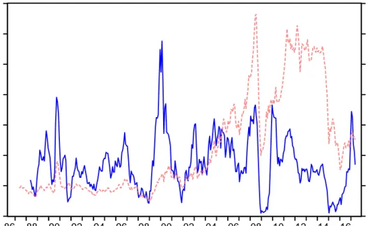
Brent price is one of reference prices for crude oil spot prices taken from the US Energy Administration. Moreover, Brent is more suitable relative to WTI prices, when investigating crude oil market with the perspective of Turkey. We are interested in the volatility of prices by using ARCH models with autoregressive mean equation. Therefore, one-year change rate of price, _{𝑏𝑟𝑒𝑛𝑡}𝑏𝑟𝑒𝑛𝑡𝑡

𝑡−12 − 1, is used as dependent variable

for the mean equation (equation [3.1]) rather that price itself, since ARCH model requires I(0) series. Time series of Brent price is taken from 1987 of May to 2017 of July (see in Figure 1). We use monthly data to examine year-to-year-volatility of variables in month of each year.

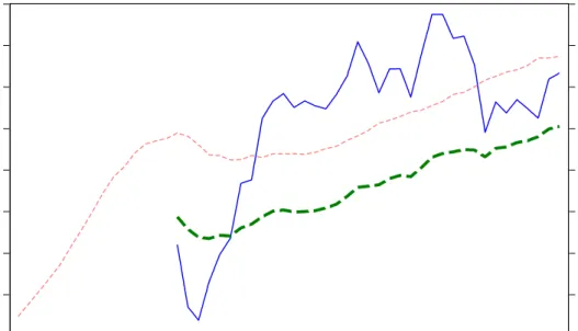
To explain the oil price dynamics, we do also include a set of explanatory variables to the mean equation. The explanatory variables are refinery utilization rate, proven reserves of natural gas, proven reserves for oil, consumption and production ratios of natural gas relative to oil. Here, refinery utilization (𝑟𝑢𝑡−1) is defined amount of

refined oil relative to capacity of oil (see Figure 2). this is a relevant variable because operating a refinery is a very costly activity and there are some economies of scale (upper bound) and lower bound to make profit (breakeven point). Price of crude oil directly affects capacity utilization of refineries or new capacity construction as investment decision.

(23)

12 0.4 0.8 1.2 1.6 2.0 2.4 2.8 3.2 0 20 40 60 80 100 120 140 86 88 90 92 94 96 98 00 02 04 06 08 10 12 14 16

GBRENT (left axis)

Brent (right axis)

Figure 1: Brent Prices

Moreover, storage of crude oil is costly too, namely, there should be demand of oil to refine and sell it immediately to make profit. It is argued that there is nonlinearity of relation between oil prices and refinery utilization by using US data (Kaufmann, Dees, Gasteuil, & Mann, 2008). As a consequence, we believe that this relation can take place with the world data and may reflect cost-profit oriented decisions of oil production. Refinery utilization data is formed from 𝑟𝑒𝑓𝑖𝑛𝑒𝑟𝑦 𝑡ℎ𝑟𝑜𝑢𝑔ℎ𝑝𝑢𝑡_{𝑟𝑒𝑓𝑖𝑛𝑒𝑟𝑦 𝑐𝑎𝑝𝑎𝑐𝑖𝑡𝑦} that are taken

from Statistical Review of World-Energy underpinning data 1965-2016 which is released by BP Energy. Frequency of data is annual in the resource but we use linear interpolation method to convert the data to monthly frequency.

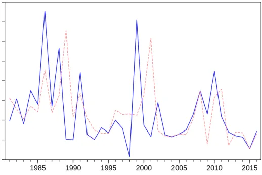
In addition, we add proven reserves of natural gas (𝑛𝑔𝑟𝑒𝑠_𝑡−1) and oil (𝑜𝑖𝑙𝑟𝑒𝑠_𝑡−1) for the purpose of defining production and consumption relation of natural gas and oil in terms of cost-profit reflection as in the refinery utilization.

(24)

13 30,000 40,000 50,000 60,000 70,000 80,000 90,000 100,000 110,000 .70 .72 .74 .76 .78 .80 .82 .84 .86 65 70 75 80 85 90 95 00 05 10 15

ref-utilization rate (right axis) ref-capacity (left axis) ref-throughput (left axis)

Figure 2: Refinery Utilization

Furthermore, because proven reserves is a function of technology and price of commodity (EIA, 2015), changes in proven reserves might reflect expectation about share of oil and natural gas in energy mix. Respectively, increasing proven reserves means investment on technology to state amount of natural gas which is able to drill the energy sources. This also can reflect substitution effect between oil and natural gas and provide a support for results from ratios. Proven reserves of natural gas and oil are also taken from Statistical Review of World-Energy underpinning data 1965-2016 (see in Figure 3) which is released from BP Energy as annual data. We employ linear interpolation to increase frequency, and use reserves ratios as follows,

𝑛𝑎𝑡𝑢𝑟𝑎𝑙 𝑔𝑎𝑠 𝑟𝑒𝑠𝑒𝑟𝑣𝑒𝑠𝑡 𝑛𝑎𝑡𝑢𝑟𝑎𝑙 𝑔𝑎𝑠 𝑟𝑒𝑠𝑒𝑟𝑣𝑒𝑠𝑡−12 and

𝑜𝑖𝑙 𝑟𝑒𝑠𝑒𝑟𝑣𝑒𝑠𝑡

𝑜𝑖𝑙 𝑟𝑒𝑠𝑒𝑟𝑣𝑒𝑠𝑡−12. So, interpolation could not alter properties

(25)

14 0.98 1.00 1.02 1.04 1.06 1.08 1.10 1.12 1.14 1985 1990 1995 2000 2005 2010 2015 OILRES-growth NGRESG-growth

Figure 3: Growth of Proven Reserves

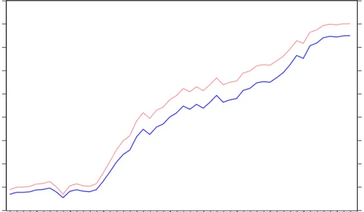
Lastly, we use four ratios to capture change in share of natural gas relative to oil in the energy mix. We construct these four measures with production volume and consumption volume in tones from Statistical Review of World-Energy underpinning data 1965-2016. These volumes also are interpolated to form variables prod1, prod2, con1 and con2. We do not use growth of these ratios since we need to relative use of gas and oil. If we add growth as in the other variables, we might lose ability of comment on ratio, because, we cannot know that this increase cause whether from rise of natural gas or fall of oil volume.

Prod1 and con1 ratios are constructed to capture relative change on natural gas according to oil. These ratios give information about reflection of consumers and producer both for oil and natural gas. Production and consumption of oil are always more than natural gas, so it is less than one through time series. Thus, we can easily capture whether natural gas and oil has correlation in movements of production and consumption with the change in value of ratios. Prod1 and con1 are defined as follows;

𝑝𝑟𝑜𝑑1 =𝑝𝑟𝑜𝑑𝑢𝑐𝑡𝑖𝑜𝑛 𝑣𝑜𝑙𝑢𝑚𝑒 𝑜𝑓 𝑁𝐺 𝑖𝑛 𝑜𝑖𝑙 𝑒𝑞𝑢𝑖𝑣𝑎𝑙𝑒𝑛𝑡

𝑝𝑟𝑜𝑑𝑢𝑐𝑡𝑖𝑜𝑛 𝑣𝑜𝑙𝑢𝑚𝑒 𝑜𝑓 𝑜𝑖𝑙

𝑐𝑜𝑛1 =𝑐𝑜𝑛𝑠𝑢𝑚𝑝𝑡𝑖𝑜𝑛 𝑣𝑜𝑙𝑢𝑚𝑒 𝑜𝑓 𝑁𝐺 𝑖𝑛 𝑜𝑖𝑙 𝑒𝑞𝑢𝑖𝑣𝑎𝑙𝑒𝑛𝑡

(26)

15 .35 .40 .45 .50 .55 .60 .65 .70 .75 .80 .26 .28 .30 .32 .34 .36 .38 .40 .42 .44 70 75 80 85 90 95 00 05 10 15

con1 (left axis) con2 (right axis)

Figure 4: Consumption Ratios

We also employ con2 and prod2 ratios to capture how production and consumption of natural gas change according to main energy consumption and production in total. Since oil have biggest share in the energy mix and natural gas is the second one, they are placed in the denominator as sum. By the ratios, we capture rise of importance of natural gas and substitution effect of natural gas. As the other ratios, these are also less than 1. 𝑝𝑟𝑜𝑑2 = 𝑝𝑟𝑜𝑑𝑢𝑐𝑡𝑖𝑜𝑛 𝑣𝑜𝑙𝑢𝑚𝑒 𝑜𝑓 𝑁𝐺 𝑖𝑛 𝑜𝑖𝑙 𝑒𝑞𝑢𝑣𝑎𝑙𝑒𝑛𝑡 𝑝𝑟𝑜𝑑𝑢𝑐𝑡𝑖𝑜𝑛 𝑣𝑜𝑙𝑢𝑚𝑒 𝑜𝑓 𝑁𝐺 𝑖𝑛 𝑜𝑖𝑙 𝑒𝑞𝑢𝑣𝑎𝑙𝑎𝑛𝑡 + 𝑝𝑟𝑜𝑑𝑢𝑐𝑡𝑖𝑜𝑛 𝑣𝑜𝑙𝑢𝑚𝑒 𝑜𝑓 𝑜𝑖𝑙 𝑐𝑜𝑛2 = 𝑐𝑜𝑛𝑠𝑢𝑚𝑝𝑡𝑖𝑜𝑛 𝑣𝑜𝑙𝑢𝑚𝑒 𝑜𝑓 𝑁𝐺 𝑖𝑛 𝑜𝑖𝑙 𝑒𝑞𝑢𝑖𝑣𝑎𝑙𝑒𝑛𝑡 𝑐𝑜𝑛𝑠𝑢𝑚𝑝𝑡𝑖𝑜𝑛 𝑣𝑜𝑙𝑢𝑚𝑒 𝑜𝑓 𝑁𝐺 𝑖𝑛 𝑜𝑖𝑙 𝑒𝑞𝑢𝑣𝑎𝑙𝑒𝑛𝑡 + 𝑐𝑜𝑛𝑠𝑢𝑚𝑝𝑡𝑖𝑜𝑛 𝑣𝑜𝑙𝑢𝑚𝑒 𝑜𝑓 𝑜𝑖𝑙

(27)

16 .35 .40 .45 .50 .55 .60 .65 .70 .75 .20 .24 .28 .32 .36 .40 .44 .48 .52 1970 1975 1980 1985 1990 1995 2000 2005 2010 2015

prod1 (left axis) prod2 (right axis)

Figure 5: Production Ratios

As we see in the Figure 4 and Figure 5, these ratios have an upper trend for the time period that we use. Thus this shows the rise of share of natural gas relative to oil and relative to energy mix. Consumption ratios also reveal a similar pattern. Thus, we can say that demand of natural gas rising regularly. On the other hand, production ratios intersect with each other and prod1 ratio increase faster than prod2. This graph suggests that source of rise in the prod1 is not only change in natural gas but it is caused by decline in production of oil as well.

(28)

17

CHAPTER 4 EMPIRICAL EVIDENCE

4.1 Benchmark Model Analysis

As mentioned above the purpose of this research is to investigate the relation between natural gas and oil price volatility. In this chapter, we present our main results in Table 2. Table 2 reports the estimates for ARCH (1) specification as in equation [3.1] and [3.3]. There are three panels where panel A illustrates mean equation results, panel B shows estimations of variance equation and lastly, panel C reports the robustness statistics. The base model which is in the first column varied through equation 15. We aim to reveal that how a change in natural gas consumption and change in supply affects the oil prices and oil price volatility. In order to capture the importance of natural gas and changes in LNG market in this relation, we employ four different measures of natural gas share of energy mix. As LNG consumption is in the natural gas consumption, we do not need LNG data separately. These ratios are Prod1, Prod2, Con1 and Con2.

Annual growth of Brent price is the dependent variable. In order to capture dynamics of the Brent prices, we use an autoregressive model. Schwarz Information Criterion (SIC)1 suggests that the order is equal to 2, then we use AR(2) model in our mean equation. As general analysis of estimation results, column 1 in table 2 provides the basic equation that captures the dynamics oil prices with lagged prices in panel A.

1_{SIC is also called Bayesian information criterion, provides penalty for loss of degrees of}

freedom. SIC = ln (u′u_T) +KlnT_T where T is number of observations and K is number of variables. The lowest value of SIC gives us this much lag in AR process gives best model(Greene, 2012).

(29)

18

Meanwhile, column 1 in panel B reveals that estimated coefficient for prod1 is negative and statistically significant. This result suggests that higher share of the natural gas production over oil production decreases the volatility of oil prices. The second column repeats the same exercise but also includes refinery utilization in mean equation. Refinery utilization helps to capture cost-profit perspective of oil production process, we explain this relation in detail above, but we extract cost-benefit oriented decision and try to capture fully substitution effect of natural gas. It is noteworthy that coefficient of production ratio in the variance equation is still negative. Continually, third equation which has different variable, which is prod1 ratio in the mean equation, panel B part of the equation investigates Prod1 ratio in the same way. Estimated coefficients of prod1 ratio are all negative and nine coefficients out of fifteen are significant. Thus, we have robust results for production ratio estimation and analysis.

On the other hand, estimated coefficients of prod1 are not significant for six specifications out of fifteen. All specifications had insignificant coefficient include refinery utilization as an explanatory variable in the mean equation. As you see in Table 1, refinery throughput and prod1 is highly correlated. As a result of this, prod1 and refinery utilization is moderately correlated. Thus, why we have insignificant estimated results might be multi-collinearity problem.

To validate our conclusion, further, we analyze each variable and their coefficients in detail, as follows. The coefficient of the first lag of price variable has a positive sign and is statistically significant at the 1 percent level. This means that inflation from the previous term based on the last year tends to influence current price growth positively. On the other hand, we observe reverse relation with second lag of oil price growth and current value for dependent variable. This might be about expectation on prices such that; increase in the price for current period can cause delays, moreover it decreases demand for oil, then it might affect future prices.

Table 1 : Correlation Table

Ref-utilization Prod1 Oilres Ngres Ref-throughput

Ref-utilization 1.000 0.589 -0.351 -0.193 0.673

Prod1 0.589 1.000 -0.293 -0.376 0.957

Oilres -0.351 -0.293 1.000 0.389 -0.360

Ngres -0.193 -0.376 0.389 1.000 -0.405

(30)

19

As mentioned in the previous chapter, refinery utilization may have a nonlinear relation with oil prices because there is a level for starting to make profit (breakeven point). In all equations, we observe that when value of refinery utilization is increasing beyond this level, it increases growth of oil prices. Therefore, rise in the utilization cause decline in growth of Brent price after this level. Furthermore, growth in refinery utilization may be proxy of increasing demand and scarcity of refined oil beyond economies of scale, thus it increases growth in prices again.

Proven reserve of oil has a positive sign in specifications 6, 7, 12, 14 and are statistically significant. A rise in proven reserves may imply increase in technology and increase in price in the previous periods. Moreover, it also implies that there was investment on oil to produce more in previous periods. In order to cover this cost, investors and producers expect to have higher prices. Thus, positive coefficient has some economic meaning. Furthermore, we have positive coefficients for proven natural gas reserve growth. Increase in proven natural gas reserves implies that investment on natural gas is increasing. Crowding out effect of investment on natural gas might occur due to substitution effect. Decline in investment on oil rises expectation on oil prices. Thus, natural gas reserves estimated with positive coefficient and it is statistically significant in specifications 4, 13, 14.

We add prod1 ratio to panel A to detect its impact on oil price directly in the mean equation. In general, we try to capture reflection of variables other than Brent price, with and without prod1 ratio. As an illustration, we examine refinery utilization with prod1 ratio in the third equation. We conclude that, increase in share of natural gas or decrease in volume of oil cause decline in prices for the third equation. On the other hand, we observe a reverse relation and have positive coefficient in equation 5 when we add natural gas reserves to the model. By looking at other equations, we see that there is a pattern. In the case of adding the natural gas reserve as natural gas production determinant, estimation output for prod1 ratio turns to positive. Thus, we might be capturing the declining oil production in prod1 ratio purely by adding natural gas reserve. Otherwise, it has a negative coefficient in general.

We add other measures to the base specification in 8, 9, 10 and 11th as it is seen in the panel A. Prod2 ratio has a positive coefficient but it is not significant in the 9th equation. We observe decrease in oil reserve more accurately with this ratio, thus increase in this ratio cause rise in the prices. Unsurprisingly, consumption ratios have

(31)

20

negative coefficients. Increasing in consumption of natural gas and decreasing consumption of oil imply decline in demand of oil, then price falls. Note that, con1 ratio is statistically significant coefficient only in the15th specification and has a negative sign.

Panel B gives information about volatility of oil prices with estimation of conditional variance. Prod1 consistently decreases uncertainty (conditional variance) in all estimation results. It has all negative sign and it is not statistically significant just for specifications 2, 3, 12, 13,14 and 15. Increasing share of natural gas in the energy mix declines volatility of oil prices. This says that if there will be alternative energy source for oil, oil prices might not volatile as much as before. Even if 1973 is not in our data, oil crises in 1973 supports our claim by showing relationship between oil prices and production volume of it. OPEC countries have an agreement on cut in supply of oil production to increase oil prices. Scarcity of oil due to decision of producer countries turned huge increase in the oil prices. As, importer countries had troubles in supply of oil to their citizens, as a resolution of troubles from supply shocks, having alternative source and supplier country might have brought energy security of countries. LNG might be this alternative source and can be substitute oil. The US and Australia have been increasing their production the market, this shows there will not be one big supplier in the future. Moreover, LNG market will be more competitive and price will have determined in the market. This substitution affect will exactly make crude oil market more competitive market as well. Namely, having more information about change in supply side of energy market declines uncertainty of oil price volatility.

Panel C reports robustness statistics of ARCH specification where we show results of application Ljung-Box Q autocorrelation test statistics2 for standardized residuals and ARCH-LM for the standardized residual3 tests. These tests identify serial correlation

2_Q LB= T(T + 2) ∑ r_j2 T−j p

j=1 has a distribution with p degrees of freedom (~χ∗2[p]). Where rj is

autocorrelation at lag j and T number of observation in the time series. null hypothesis is no autocorrelation as of lag j otherwise, data is not random. If QLB> χ∗2[p], then reject the null

hypothesis (Greene, 2012).

3_{Critical value of ARCH-LM test has chi-squared distribution and with p degrees of freedom,}

(32)

21

of standardized residuals and give idea about how our result accurate. The test statistics could not reject the null of no autocorrelation at least for first six lag in specifications 1, 4, 5, 6, 7, 8, 9, 10 and 11. Nevertheless, we do not observe auto-correlated error till at least third lag for equation with refinery utilization rate. Additionally, we fail to reject null hypothesis of ARCH-LM test for all estimated coefficients but sixth and twelfth lag which are not statistically significant. Overall, according to significance result of ARCH-LM test, we can reject the null for just first lag for the specifications 2,3,12,13,14 and 15.

Forecast error is as random variable in ARCH model, and the conditional variance is dependent variable in the panel B. Variance must not be negative, thus implies that variance equation should not be negative. To satisfy this condition, first, disturbance of variance estimation should be bounded below from negative of constant term where constant is positive. Second, roots of characteristic function should lie outside the unit circle, to be certain that this equation is not explosive. In the case of all coefficient (the ones determine relations of error terms square and conditional variance) is positive, the condition turns to be all coefficient should less than 1. Coefficients of forecast error square in the variance equation estimation are all positive in panel B. Additionally, all coefficients of disturbances of mean estimation is less than 1 and thus volatility estimation is not explosive. Furthermore, constant term is also all positive. Namely, we estimate monotonically increasing positive variance with ARCH specification, this implies our results and our models are robust.

test. Null hypothesis is no autocorrelation for first P lags. H1 states error term have AR(p) process.

Reject H0, if 𝑇𝑅∗2> χ∗2 (Greene, 2012).

(33)

22

Table 2: ARCH (variance equation with 𝒑𝒓𝒐𝒅𝟏𝒕−𝟏) 1988-2016

1 2 3 4 5 6 7 8 9 10 11 12 13 14 15 Mean Equation constant 0.060 -1892.575 -1872.619 -0.292 -0.403 -0.510 -0.509 0.055 0.052 0.083 0.092 -1998.388 -2075.243 -2140.411 -1197.299 (0.001) (0.000) (0.000) (0.240) (0.149) (0.041) (0.047) (0.335) (0.567) (0.205) (0.372) (0.000) (0.000) (0.000) (0.000) 𝒑𝒕−𝟏 1.1309*** 1.159*** 1.159*** 1.124*** 1.122*** 1.108*** 1.108*** 1.130*** 1.130*** 1.133*** 1.133*** 1.146*** 1.158*** 1.149*** 1.130*** (0.000) (0.000) (0.000) (0.000) (0.000) (0.000) (0.000) (0.000) (0.000) (0.000) (0.000) (0.000) (0.000) (0.000) (0.000) 𝒑𝒕−𝟐 -0.192*** -0.279*** -0.279*** -0.194*** -0.189*** -0.177*** -0.177*** -0.190*** -0.190*** -0.197*** -0.197*** -0.264*** -0.277*** -0.259*** -0.267*** (0.001) (0.000) (0.000) (0.001) (0.001) (0.002) (0.002) (0.001) (0.001) (0.000) (0.000) (0.000) (0.000) (0.000) (0.000) 𝒓𝒖𝒕−𝟏* 6853.444*** 6781.754*** 7238.282*** 7525.764*** 7760.371*** 4330.500*** (0.000) (0.000) (0.000) (0.000) (0.000) (0.000) 𝒓𝒖𝒕−𝟏𝟐 -8271.232*** -8185.365*** -8741.798*** -9099.060*** -9383.426*** -5220.242*** (0.000) (0.000) (0.000) (0.000) (0.000) (0.000) 𝒓𝒖𝒕−𝟏𝟑 3327.102*** 3292.832*** 3518.982*** 3666.827*** 3781.801*** 2097.869*** (0.000) (0.000) (0.000) (0.000) (0.000) (0.000) 𝒏𝒈𝒓𝒆𝒔𝒕−𝟏* 0.354 0.426* 0.634*** 0.486** 0.053 (0.152) (0.097) (0.000) (0.016) (0.437) 𝒐𝒊𝒍𝒓𝒆𝒔𝒕−𝟏* 0.568 ** _0.569** _0.843*** _0.738*** (0.020) (0.020) (0.000) (0.001) 𝒑𝒓𝒐𝒅𝟏𝒕−𝟏* -0.032447 0.053 -0.002 0.006 0.000 0.050 0.044 2.605*** (0.277) (0.539) (0.984) (0.942) (1.000) (0.530) (0.617) (0.000) 𝒑𝒓𝒐𝒅𝟐_𝒕−𝟏* _0.017 (0.939) 𝒄𝒐𝒏𝟏𝒕−𝟏* -0.029 -3.012*** (0.761) (0.000) 𝒄𝒐𝒏𝟐𝒕−𝟏* -0.073 (0.778) Variance Equation constant 0.037 0.016 0.016 0.039 0.040 0.037 0.037 0.037 0.037 0.037 0.037 0.018 0.016 0.016 0.015 (0.009) (0.317) (0.302) (0.005) (0.005) (0.005) (0.005) (0.009) (0.009) (0.009) (0.009) (0.332) (0.284) (0.247) (0.267) 𝒖𝒕−𝟏𝟐 0.357** 0.330** 0.337** 0.367** 0.369** 0.376** 0.376** 0.358** 0.358** 0.357** 0.357** 0.171** 0.391** 0.381** 0.369** (0.024) (0.022) (0.027) (0.023) (0.024) (0.023) (0.023) (0.025) (0.025) (0.024) (0.024) (0.033) (0.034) (0.023) (0.027) 𝒑𝒓𝒐𝒅𝟏𝒕−𝟏 -0.040* -0.006 -0.006 -0.043** -0.044** -0.040** -0.040** -0.040* -0.040* -0.039* -0.039* 0.000 -0.007 -0.008 -0.007 (0.059) (0.813) (0.791) (0.036) (0.032) (0.037) (0.037) (0.059) (0.059) (0.060) (0.060) (1.000) (0.745) (0.706) (0.752)

(34)

23

*_{[ru= refinery utilization (assumed as nonlinear), ngres= growth in natural gas proven reserves, oilres=growth in proven oil reserves, prod1= production of gas over production of oil in ton, prod2= production of gas over}

production of gas and oil together (in ton), con1= consumption of gas over consumption of oil (in tons), con2= consumption of gas over consumption of gas and oil together (in tons), h= conditional variance; u= error term]

1 2 3 4 5 6 7 8 9 10 11 12 13 14 15

Panel C: Robustness statistics Lag(s) Ljung-Box Q-Stat

1 1.262 0.286 0.257 1.155 1.287 1.303 1.302 1.311 1.315 1.114 1.123 0.173 0.222 0.223 0.364 (0.261) (0.593) (0.612) (0.282) (0.257) (0.254) (0.254) (0.252) (0.252) (0.291) (0.289) (0.677) (0.637) (0.637) (0.546) 3 5.710 11.049 9.763 5.777 5.852 5.539 5.536 5.723 5.724 5.693 5.694 12.940 9.494 8.524 10.128 (0.127) (0.011) (0.021) (0.123) (0.119) (0.136) (0.137) (0.126) (0.126) (0.128) (0.127) (0.005) (0.023) (0.036) (0.018) 6 6.235 11.324 10.033 6.206 6.282 7.009 7.009 6.256 6.258 6.189 6.192 14.357 9.715 9.410 10.491 (0.397) (0.079) (0.123) (0.401) (0.392) (0.320) (0.320) (0.395) (0.395) (0.402) (0.402) (0.026) (0.137) (0.152) (0.105) 12 62.117 68.786 67.800 61.482 60.986 62.784 62.802 62.077 62.076 62.240 62.227 75.780 68.277 68.461 68.394 (0.000) (0.000) (0.000) (0.000) (0.000) (0.000) (0.000) (0.000) (0.000) (0.000) (0.000) (0.000) (0.000) (0.000) (0.000) 24 107.660 106.230 67.800 105.930 105.270 109.490 109.520 107.730 107.730 107.390 107.400 114.470 108.650 108.580 108.680 (0.000) (0.000) (0.000) (0.000) (0.000) (0.000) (0.000) (0.000) (0.000) (0.000) (0.000) (0.000) (0.000) (0.000) (0.000) Lag(s) ARCH-LM tests; f-stat

1 0.134 0.131 0.194 0.142 0.135 0.152 0.152 0.132 0.132 0.142 0.142 1.440 0.399 0.392 0.374 (0.714) (0.717) (0.660) (0.707) (0.713) (0.697) (0.697) (0.717) (0.717) (0.707) (0.707) (0.231) (0.528) (0.532) (0.541) 3 0.278 2.169 1.450 0.323 0.341 0.415 0.414 0.276 0.276 0.286 0.285 6.760 1.281 1.189 2.055 (0.842) (0.092) (0.228) (0.809) (0.796) (0.742) (0.743) (0.842) (0.843) (0.836) (0.836) (0.000) (0.281) (0.314) (0.106) 6 2.140 3.031 2.790 2.221 2.121 1.642 1.643 2.124 2.123 2.204 2.200 4.629 2.977 2.222 3.110 (0.049) (0.007) (0.012) (0.041) (0.051) (0.135) (0.414) (0.050) (0.050) (0.043) (0.043) (0.000) (0.008) (0.041) (0.006) 12 1.964 2.156 2.119 2.023 1.961 1.448 1.449 1.956 1.955 1.993 1.991 3.103 2.330 1.767 2.111 (0.027) (0.014) (0.016) (0.022) (0.027) (0.143) (0.143) (0.028) (0.028) (0.025) (0.025) (0.000) (0.007) (0.053) (0.016) 24 1.161 1.293 1.256 1.141 1.115 0.894 0.894 1.159 1.158 1.168 1.167 1.772 1.276 1.017 1.112 (0.277) (0.167) (0.194) (0.298) (0.326) (0.611) (0.610) (0.280) (0.280) (0.271) (0.271) (0.016) (0.179) (0.444) (0.329) Kurtosis 5.392 5.810 5.768 5.447 5.464 5.563 5.564 5.392 5.392 5.396 5.396 6.176 5.820 5.970 6.115

(35)

24

4.2

Caveats and Future Research

In order to check robustness of our results, we perform a further set of analyses. First, we repeat the benchmark exercise with other ratios of consumption and production. Then, adequacy of ARCH specification is tested by doing benchmark estimation with EGARCH and GARCH model. Lastly, ARCH specifications are performed for various time windows to examine the robustness of estimated result over time.

Table A1, A2 and A3 repeat the benchmark exercises with the alternative definition of the natural gas shares. Table A1 uses the prod2 which has oil production as well as natural gas production in the denominator. Table A2 is included con1 ratio, which is consumption of natural gas divided by oil consumption. A3 uses con2 that purposes to capture same implication with A1 but with the consumption volumes. Basically, results of the estimated coefficient for the various natural gas share ratios has the same fashion with the benchmark model. However, we just use prod1 ratio in the benchmark model compare to others, because prod2 ratio has less volatility then prod1 ratio, so the benchmark model avoids Type II error. Considering consumption ratios, we believe that production leads the consumption of the natural gas which is resulted that consumption and production has same pattern. Thus, we provide estimations of consumption ratios to show that our results are robust.

Furthermore, robustness of our statistics validated with a the GARCH (1,1) specification. The estimated coefficient for the prod1 are all negative but none of them is statistically significant. One of the reason for this result is that, the persistency of conditional volatility may coincide with the production persistency (see figure 3.2.5). Thus, production and persistency of the conditional variance may move together and we may fail to eliminate this problem at this stage. As consequence, we rather keep ARCH (1) specification as benchmark model, because it is still efficient and consistent estimator. As further study as we discuss in the above, we perform EGARCH (1,1) specification that may validate the basic conclusion of the paper. Additionally, we can state that volatility in the results may cause by Type-I error which means result of estimations with different specification reject our hypothesis in the case that our is true.

(36)

25

Relationship between the oil price volatility and natural gas share might be changing over time, then we repeat the exercise for the benchmark specification subsamples of five years. Results are mostly parallel but the level of significance decreases drastically on the estimated coefficient of the prod1 on the conditional variance. Regarding ARCH specification and derivations are highly nonlinear systems, the computation may fail to converge relative to estimation with full sample. We get the strongest support from observations for the time windows of 1993-1997 and 1998-2002. Estimated coefficients are all negative for these periods. On the other hand, prod1 ratio in the variance equation has nine positive coefficients out of fifteen for the time period of 2003-2007, but note that all are statistically insignificant. Additionally, nonlinearity of refinery utilization fails and third level of nonlinearity do not exist for these estimations. Reason might be sharp declining in the amount of data. Moreover, estimated parameters with lower number of data are sensitive to outliers. Thus, estimated coefficient is volatile among our results.

We further perform the subsample analyses for seven years in the tables A12 to A16 and analysis for decades in A17 to A19. Results prevails that we have evidence for our claim that we gather effect of the natural gas market on the oil price volatility is negative. However, subsample stability might be questionable, it is probably due to low of degree of freedom.

Taking seven-year windows of whole data, we reached clusters of different result. As seen in table A12 and A15, prod1 ratio in the variance function has negative coefficient in general and is statistically significant for some of equations. Brent prices also have same behavior as in the fundamental analysis. We can conclude that; this part of the seven-year analysis supports our results. It is noteworthy that information in the time series of prod1 decreases the conditional variance in table A15 which covers 2008 crisis years. So that, we can claim that consumption behavior may give information of aggregate economy and it may decrease the uncertainty on oil prices. Table A13 differs from our result because of having statistically significant positive coefficient of prod1 ratio in the variance equation. This time period represents 1998 oil crisis years at which oil prices decreases sharply. Hence, production of oil cannot give unbiased information since OPEC countries failed to agree on cut of supply that create great uncertainty in prices. Namely, the estimated coefficient of prod1 ratio may differentiate specifically

(37)

26

for these years. Slope difference of prod1 and prod2 ratio is increasing for years of A14 and A16 (see in figure 3.2.5), inconsistency of coefficient in prod1 may occurred by the fact that.

As a consequence, having short run fluctuations may not give substitution effect of natural gas and oil. Since substitution is exactly result of long-run relation. We may not capture long-run movement of data, but results can be biased with shocks and short-run cycles.

In the near future, we are planning to address these unsolved problems of estimations and try different methods and specifications. As an illustration, we may use threshold GARCH methods to estimate this relation. In order to get rid of non-linearity of (G)ARCH models, we may focus specifically on various regions by using their consumptions/production volumes of natural gas and oil, establish prod1, prod2, con1 and con2 ratios for these regions. Thus, we can investigate relations of oil price and oil price volatility with these ratios by using (G)ARCH specification.

It is believed that natural gas and LNG may have an impact on oil price volatility via impulse (𝑢_𝑡−12 _{) or persistency (ℎ}

𝑡−1

2 _{) , so we can try specification with these variable}

in the variance function, such that; ℎ_𝑡2 _{= 𝛿 + 𝛼}

1𝑢𝑡−12 + 𝛼2𝐼𝑡𝑢𝑡−12 + 𝛽ℎ𝑡−12 [4.1]

or

ℎ_𝑡2 _{= 𝛿 + 𝛼}

1𝑢𝑡−12 + 𝛽1ℎ𝑡−12 + 𝛽2𝐼𝑡ℎ𝑡−12 [4.2]

where “I” is an impulse dummy.

As an additional exercise, we have data set between 1988 and 2017 which is time period that has clusters with high inflation. We may repeat our study with real oil prices again.

Note that one may argue that, the reason of decline in conditional variance of oil prices is not higher share of natural gas in energy market but it is lower oil prices. On the other hand, it is might be argued that the reason decrease in oil prices could be higher natural gas shares in the market. Nevertheless, we can follow two exercises as including lagged values of oil prices (but not growth) to the variance equation, or, as using ℎ𝑡2⁄𝑝𝑡−1 instead of ℎ𝑡2 in the variance equation.

(38)

27

CHAPTER 5 CONCLUDING REMARKS

This research aims to estimate the relation between share of natural gas in the energy market and oil price volatility. Natural gas and oil substıtutes each other but they have also different features in terms of market structure. Oil is traded in the competitive market and it is also financial commodity. But natural gas is not easy to store and transportation is more difficult relative to oil. In the light of these facts, we can claim that substitution effect can be improved with the developing LNG market and with increase in supply of natural gas. How volatility of oil affected are; first, energy market will be more secure due to having alternative to oil dependency of oil decreases then uncertainty on oil prices will decrease, second decline in demand due to environmental policies and having more elastic demand because of having alternative source for inventories, makes LNG is more attractive. Then oil price volatility may decrease again. To summarize, we believe that change in energy mix influences role of oil in energy market and decreases oil price volatility.

There might be other alternative sources to substitute oil and we avoided here. Share of natural gas and oil is %80 percent in the world primary energy sources, rest includes coal and clean energy sources. As a discussion for other alternatives to oil in energy mix, we should state that renewable energies such hydropower, nuclear energy, wind and solar power. Hydropower and nuclear power provides constant stream of clean energy. Therefore, energy production in hydropower is restricted with physical constraints to be substitute other energy sources, even if it is cheap. Additionally, solar and wind power are too expensive and cannot provide constant energy production. However, as they substitute oil in electricity generation, we can

(39)

28

state that there might be impacts of these sources on oil prices and more importantly oil price volatility.

Nuclear power is cheapest clean energy source, which is used in 11% of electricity generation in the world, but it is more expensive than oil, oil derivatives and natural gas. The important question is that, can nuclear power be substitute oil consumption. according to Toth and Rogner (2006), it is not possible for today’s world, because natural gas, coal and nuclear power have competed with oil for power generation, hence, natural gas is the primary source in power generation now. In order to switch oil to nuclear power, industries should make additional investment on production process and government should give subsidies to support this environmentally friendly switching. Maybe they can substitute each other in the future as much as affecting oil prices. A further set of studies, it might be performed as study that we perform here, regarding the role of natural gas on oil for hydra-power, nuclear power, sun and wind energies rather than natural gas.

We investigate relationship between natural gas and oil price volatility with different time series model specifications but ARCH model is mainly used in our analysis. We use time series of monthly Brent price in between 1987-2017 as dependent variable with ARCH specification to capture price volatility. We add 4 different measures of production and consumption for relative changes in oil and natural gas. Main argument concluded from empirical findings is increasing in the production of natural gas or decreasing in production of oil cause decline in oil price volatility. This paper represents the empirical results and analyze estimated models in detail. These changes in production are resulted from substitution effect and we discuss arguments on channels of this effect. Namely, energy security, environmental policies and inventories can be reason of this changes in the market structure

Our question is very important, because variance in the market can change balance of the energy diplomacy. Moreover, the main concern of energy importing countries, energy security, can be released with the substitution of energy commodities. In order to observe full deviation in the energy market, maybe we would have need more time to have more data. But natural gas market analysts clearly state that the time of LNG will come.

(40)

29

REFERENCES

Alterman, Sofya. (2012) . Natural gas price volatility in the UK and North America.

Asche, F., Osmundsen, P., & Sandsmark, M. (2006). The UK market for natural gas, oil and electricity: are the prices decoupled?. The Energy Journal, 27-40.

Bachmeier, L. J., & Griffin, J. M. (2006). Testing for market integration crude oil, coal, and natural gas. Energy Journal, 27(2), 55–71.

https://doi.org/10.5547/ISSN0195-6574-EJ-Vol27-No2-4

Brigida, M. (2014). The switching relationship between natural gas and crude oil

prices. Energy Economics, 43, 48-55.

Brown, S. P., & Yücel, M. K. (2008). What drives natural gas prices?. The Energy Journal, 45-60.

Chedid, R., Kobrosly, M., & Ghajar, R. (2007). A supply model for crude oil and natural gas in the Middle East. Energy Policy, 35(4), 2096-2109.

Economides, M. J., Oligney, R. E., & Lewis, P. E. (2012). US natural gas in 2011 and beyond. Journal of Natural Gas Science and Engineering, 8, 2-8. EIA, U. (2016). Crude Oil and Natural Gas Proved Reserves Year-end 2015. Ewing, B. T., Malik, F., & Ozfidan, O. (2002). Volatility transmission in the oil and

natural gas markets. Energy Economics, 24(6), 525-538.

Greene, W. H. (2018). Econometric analysis. New York, NY: Pearson

(41)

30

Hartley, P. R., Medlock III, K. B., & Rosthal, J. E. (2008). The relationship of natural gas to oil prices. The Energy Journal, 47-65.

Kaufmann, R. K., Dees, S., Gasteuil, A., & Mann, M. (2008). Oil prices: the role of refinery utilization, futures markets and non-linearities. Energy

Economics, 30(5), 2609-2622.

Krichene, N. (2002). World crude oil and natural gas: a demand and supply model. Energy Economics, 24(6), 557-576.

Medlock III, K. B., & Hartley, P. R. (2010, October). Shale gas and emerging market dynamics. In USAEE/IAEE’s 29th North American Conference. Calgary, Alberta: James A Baker III Institute for Public Policy Rice University. Miyazaki, K., & Limam, M. (2013, May). Will LNG exports from North

America/East Africa drive global price integration?. In 17th International Conference & Exhibition on Liquefied Natural Gas (LNG 17).

Mu, X. (2007). Weather, storage, and natural gas price dynamics: Fundamentals and volatility. Energy Economics, 29(1), 46-63.

Muth, J. F. (1961). Rational expectations and the theory of price

movements. Econometrica: Journal of the Econometric Society, 315-335. Neumann, A. (2009). Linking natural gas markets–is LNG doing its job?. The

Energy Journal, 187-199.

Özdemir, Volkan (2017). Doğal Gaz Piyasaları; Türkiye Enerji Güvenliği Üzerine Tezler (1st ed.). Istanbul: Kaynak Yayınları

Pindyck, R. S. (2004). Volatility in natural gas and oil markets. The Journal of Energy and Development, 30(1), 1-19.