SIMULATION OF STEADY-STATE RESPONSE OF
TIP-SAMPLE INTERACTION FOR A TORSIONAL
CANTILEVER IN TAPPING MODE ATOMIC FORCE
MICROSCOPY FOR MATERIAL
CHARACTERIZATION IN NANOSCALE
a thesis
submitted to the department of electrical and
electronics engineering
and the institute of engineering and science
of bilkent university
in partial fulfillment of the requirements
for the degree of
master of science
By
S¸eref Burak Selvi
August 31, 2010
I certify that I have read this thesis and that in my opinion it is fully adequate, in scope and in quality, as a thesis for the degree of Master of Science.
Prof. Dr. Abdullah Atalar (Supervisor)
I certify that I have read this thesis and that in my opinion it is fully adequate, in scope and in quality, as a thesis for the degree of Master of Science.
Prof. Dr. Hayrettin Koymen
I certify that I have read this thesis and that in my opinion it is fully adequate, in scope and in quality, as a thesis for the degree of Master of Science.
Asst. Prof. Dr. Coskun Kocabas
Approved for the Institute of Engineering and Science:
Prof. Dr. Levent Onural
Director of the Institute Engineering and Science
in loving memory of my family
ABSTRACT
SIMULATION OF STEADY-STATE RESPONSE OF
TIP-SAMPLE INTERACTION FOR A TORSIONAL
CANTILEVER IN TAPPING MODE ATOMIC FORCE
MICROSCOPY FOR MATERIAL
CHARACTERIZATION IN NANOSCALE
S¸eref Burak Selvi
M.S. in Electrical and Electronics Engineering Supervisor: Prof. Dr. Abdullah Atalar
August 31, 2010
Dynamic atomic force microscopy (AFM) techniques involving multifrequency excitation or detection schemes offer improved compositional sensitivity and quantitative material property imaging. A correct interpretation of cantilever vibrations in multifrequency excitation and detection schemes demands an im-proved understanding of the effects of enhanced high frequency vibrations on the steady-state dynamics of the cantilever and in particular, on the tip-sample interaction force.
In this thesis, a simulation background is developed with proper modelling of tip-sample ensemble for accurate simulation of tip-sample interaction when mul-tifrequency excitation and detection schemes are utilized. The simulation results are analyzed and used for material characterization. The tip-sample ensemble is modelled as a multiple degree of freedom system that includes torsional mode and higher order flexural modes of the cantilever. The nonlinear behavior of sample surface is also included in the model. This mechanical model is transformed into an electrical circuit and an electrical circuit simulator is used to find steady-state of the circuit. Thereby, a simulation of steady-state dynamics of multifrequency imaging schemes is achieved.
Using the developed simulation tool, the effect of torsional vibrations and higher order flexural vibrations on steady-state of tip-sample interaction is in-vestigated. The tip trajectory and tip-sample interaction force are calculated for torsional harmonic cantilevers. The potential of torsional harmonic cantilevers in reconstruction of tip-sample interaction force for the quantitative estimation of
v
material properties is verified. Change in amplitude of torsional harmonics with respect to elastic modulus (sensitivity) is investigated. It is shown that sensitiv-ity of a particular torsional harmonic changes with sample stiffness and higher harmonics are more sensitive to change in stiffness. Additionally, a noise analysis of torsional harmonic cantilevers is made and included in the simulations. The tip-sample interaction force is recovered from the simulated torsional vibration signal and the effective elastic modulus of the sample is estimated. It is observed that accuracy of the estimation is affected by number of torsional harmonics used in the recovery of interaction force.
Keywords: Atomic force microscope, torsional harmonic cantilever, harmonic imaging, multifrequency imaging, tip-sample interaction, material characteriza-tion.
¨
OZET
NANO ¨
OLC
¸ EKTE MATERYAL KARAKTER˙IZASYONU
˙IC¸˙IN VURMA MODU ATOM˙IK KUVVET
M˙IKROSKOB˙IS˙INDE TORS˙IYONEL KALDIRAC
¸
KULLANILDI ˘
GINDA UC
¸ -Y ¨
UZEY ETK˙ILES¸˙IM˙IN˙IN
DENGE DURUMU DAVRANIS¸ININ S˙IM ¨
ULASYONU
S¸eref Burak Selvi
Elektrik ve Elektronik M¨uhendisli˘gi, Y¨uksek Lisans Tez Y¨oneticisi: Prof. Dr. Abdullah Atalar
31 A˘gustos 2010
C¸ oklu frekansta eksitasyon ve deteksiyon y¨ontemlerini kullanan dinamik atomik kuvvet mikroskopi teknikleri normalden daha iyi madde kompozisyonu du-yarlılı˘gı sa˘glamakta ve materyal ¨ozelliklerinin kuantitatif olarak g¨or¨unt¨ulenmesini olanaklı kılmaktadır. C¸ oklu frekans eksitasyon ve deteksiyon y¨ontemleri kul-lanıldı˘gında elde edilen kaldıra¸c titre¸simlerinin do˘gru anlamlandırılabilmesi i¸cin g¨u¸clendirilmi¸s y¨uksek frekanslı titre¸simlerin kaldıra¸c ve u¸c-y¨uzey kuvvetine etk-isinin iyice anla¸sılması gerekmektedir.
Bu tezde, ¸coklu eksitasyon ve deteksiyon y¨ontemleri kullanıldı˘gı zaman u¸c-y¨uzey sisteminin davranı¸sının aslına uygun hesaplanabilmesi i¸cin bir sim¨ulasyon altyapısı olu¸sturuldu. Sim¨ulasyon sonu¸cları y¨uzeydeki maddelerin karakterizasy-onu i¸cin kullanıldı. U¸c-y¨uzey birlikteli˘gi, kaldıracın torsiyonel modu ile y¨uksek fleksiyonel modlarının da hesaba katıldı˘gı bir ¸coklu serbestlik derecesi sistemi olarak modellendi. Y¨uzeyin do˘grusal olmayan (nonlineer) davranı¸sına da mod-elde yer verildi. Mekaniksel bu model bir elektrik devresine transform edildi ve devrenin kararlı durumu devre sim¨ulat¨or¨u kullanılarak ¸c¨oz¨uld¨u. Bu sayede ¸coklu frekans g¨or¨unt¨ulemenin kararlı durumunun sim¨ulasyonu yapılmı¸s oldu.
Geli¸stirilen sim¨ulasyon aracı kullanılarak torsiyonel titre¸simlerin ve y¨uksek seviye fleksiyonel titre¸simlerin u¸c-y¨uzey etkile¸simine olan etkisi ara¸stırıldı. U¸c y¨or¨ungesi ve u¸c-y¨uzey etkile¸sim kuvveti torsiyonel kaldıra¸clar i¸cin hesap-landı. Kuantitatif materyal karakterizasyonuna torsiyonel kaldıra¸cların mukte-dir oldu˘gu sonu¸clarla desteklendi. Y¨uzey sertli˘gine g¨ore torsiyonel harmoniklerin
vii
b¨uy¨ukl¨uklerindeki de˘gi¸sim ara¸stırıldı. Torsiyonel harmonikler y¨uzey sertli˘gine du-yarlı oldu˘gu ve bu dudu-yarlılı˘gın y¨uksek torsiyonel harmoniklere gidildik¸ce daha da arttı˘gı g¨or¨uld¨u. Bunlara ek olarak torsiyonel kaldıra¸clar i¸cin g¨ur¨ult¨u analizi de yapıldı ve modele eklendi. Sim¨ulasyon sonucunda ¸cıkan torsiyonel titre¸sim sinyali kullanılarak u¸c-y¨uzey etkile¸sim kuvveti hesaplandı ve bu hesaplanan sinyalden y¨uzey sertli˘gi parametresi kestirildi. Kestirimin do˘grulu˘gunun etkile¸sim kuvvetini geri hesaplamada kullanılan torsiyonel harmonik sayısı ile do˘gru orantılı oldu˘gu g¨or¨uld¨u.
Anahtar s¨ozc¨ukler : Atomik kuvvet mikroskobu, torsiyonel harmonik kaldıra¸c, harmonik g¨or¨unt¨uleme, ¸cok frekanslı g¨or¨unt¨uleme, u¸c-y¨uzey etkile¸simi, materyal karakterizasyonu.
ACKNOWLEDGEMENTS
I would like to express my sincere gratitude to Dr.Abdullah Atalar for his supervision, guidance and encouragement through the development of this the-sis. Besides the academic and ethic stance, I have grasped much about success, patience, humility, diligence, leadership, versatility and many more from him in the last three years. I believe that these tenets will brighten my way in the rest of my life.
I would like to thank to the members of my thesis jury for reading the manuscript and commenting on the thesis.
Endless thanks to officemates and group members Vahdettin Tas, Mehmet Deniz Aksoy, Kaan Oguz, Selim Olcum, Mehmet Niyazi Senlik and Elif Aydogdu for useful discussions. Many thanks to Kemal Gurel, Halil Ibrahim Sahin, Mursel Yildiz, Mehmet Can Kerse, Ahmet Emrah Sezgin, Fazli Kaybal, and Mert Vural for filling nonresearch times with full of fun.
I especially thank to my family for their support and love. Without the sup-port of my parents, this work would never be possible. My mother Sengun and my father Yusuf have strived for making life easier for me so that I could focus on my education. I also thank my sister Ilknur and her husband Fırat for their support and friendship.
Finally, special thanks to Ozgur Sahin who incite me to research on this in-teresting topic by accepting me as a summer trainee for the research program at Harvard when I was just a junior student at Bilkent. That experience is a milestone in my life.
I acknowledge the financial aid of Turkish Republic, the 2228 and 2224 schol-arships of TUBITAK.
Contents
1 INTRODUCTION 1
2 SIMULATION BACKGROUND 4
2.1 Overview of the Overall System . . . 4
2.2 Torsional Harmonic Cantilever . . . 6
2.3 The Model . . . 7
2.4 Tip-Sample Interaction . . . 10
2.5 Noise Analysis . . . 13
2.6 Implementation of the Overall System as an Electrical Circuit . . 16
2.6.1 Drive Circuit . . . 18
2.6.2 Equivalent Circuit of the First Three Flexural Modes of the Cantilever . . . 19
2.6.3 Equivalent Circuit of the First Torsional Mode of the Can-tilever . . . 20
2.6.4 Equivalent Circuit of the Sample Surface . . . 21
2.6.5 Feedback Circuit . . . 22 ix
CONTENTS x
2.6.6 Photodetector Circuit . . . 23
3 SIMULATION RESULTS 24
3.1 Effect of the Enhanced Higher Order Vibrations on Steady-State Dynamics . . . 24 3.2 Material Characterization with the Torsional Harmonic
Can-tilevers in the Presence of Noise . . . 33
List of Figures
2.1 Typical tapping mode atomic force microscopy. The elements of the system are given in the figure. . . 5 2.2 Vibration modes of a torsional harmonic cantilever. (a) No
exci-tation, (b) first flexural mode is excited, (c) first torsional mode is excited, (d) first flexural and first torsional modes are both excited. 7 2.3 Coordinate system for the overall tip deflection of the torsional
har-monic cantilever. The total deflection of the cantilever (z) on the tip side is assumed as the summation of the flexural (zf) and
tor-sional (zt) deflections of the cantilever. The surface displacement
(zs) is included in the model. Note that zf =!izi and zt=!jz˜j.
Positive direction for the vectors of force and deflection is depicted in the figure. . . 8 2.4 Electrical equivalent circuit of the multiple degree of freedom
model of the tip-sample ensemble. The variables with tilde over them represents the torsional variables. Each of the vibrational modes is represented by a series RLC circuit where the sample surface is represented by a RC circuit. . . 10 2.5 Fts vs. (z− zs). After the contact is established in the oscillation
cycle, as tip indents the surface, (z− zs) stars to shrink from ao
to zero and Fts quickly reaches the value that needed to push the
surface inwards and keeps z− zs ≈ ao. . . 12
LIST OF FIGURES xii
2.6 Equivalent noise circuit of the system consists of the photodetector, the cantilever and the transimpedance amplifier. is, ish, im, en, in,
eR represent the sources corresponding to the output signal of the
photodetector, shot noise of the photodetector, thermomechanical noise of the cantilever, input noise voltage of the transimpedance amplifier, input noise current of the transimpedance amplifier and Johnson noise voltage of the transimpedance amplifier, respectively. 14 2.7 Block diagram of the overall circuit. . . 17 2.8 Circuit that is used to drive the cantilever in its first flexural
res-onant mode. . . 18 2.9 Equivalent circuit of the first three flexural modes of the cantilever. 19 2.10 Equivalent circuit of the first torsional mode of the cantilever. . . 20 2.11 Equivalent circuit of the sample surface. . . 21 2.12 Feedback circuit part of the overall circuit. . . 22 2.13 Photodetector circuit. . . 23
3.1 Tip displacement and surface motion in the case of (a) compliant and (b) stiff sample after three Q1 cycles. Note that z−zsis always
greater than zero. There is a hysteresis in the surface elongation (depicted by star on the figure) because of energy dissipation. . . 27 3.2 Torsional vibrations on the torsional harmonic cantilever in the
case of (a) compliant and (b) stiff sample after three Q1 cycles. . 28 3.3 Harmonics of the torsional vibrations up to the resonance of the
torsional mode in the case of (a) compliant and (b) stiff sample after three Q1 cycles. Axis limit of y-coordinate is not preserved because of illustration purposes. Star is used to depict the first zero crossing of the magnitude of the harmonics. . . 29
LIST OF FIGURES xiii
3.4 Actual tip-sample interaction force and recovered one from first 16 torsional harmonics in the case of (a) compliant and (b) stiff sample after three Q1 cycles. . . 30 3.5 Change in magnitude of various harmonics of the torsional
vibra-tions with respect to the effective elastic modulus . . . 32 3.6 Simulation outcomes for a sample with E∗=100MPa, H=5e-20J
a) noisy photodetector signal (N=50) b) recovered TSIF (M=15), estimated E∗ is 98.495MPa c)spectrum of b) . . . . 36
3.7 Estimations over a wide range of materials in the presence of noise. Estimations with M=15 are depicted by circles. Estimations that the harmonics up to the first zero crossing of the spectrum of TSIF is used are depicted by dots. . . 37
Chapter 1
INTRODUCTION
Atomic force microscope [1] (AFM) is one of the most commonly used imag-ing tools in nanotechnology. Among the imagimag-ing modes of AFM, tappimag-ing mode (TM) [2] is widely used especially on soft samples, because the gentle interac-tion forces can be achieved (peak forces as low as 600pN) [3], it enables a high spatial resolution and results in less lateral interaction compared to the other imaging modes [4]. In this mode, AFM cantilever is excited at or near its funda-mental resonance frequency and the tip experiences a nonlinear interaction force periodically. This periodic nonlinear force gives rise to the vibrations on the cantilever that are at the integer multiples (higher harmonics) of the excitation frequency [5].
The topography of the sample surface and the phase of the first flexural har-monic are measured in a typical TM-AFM imaging. The topography and the phase are not sufficient alone to extract the material properties of a given sam-ple, because the measured parameters (the amplitude and the phase of the first harmonic of the cantilever motion) provide only a time averaged value of the tip-sample interaction force (Fts) [5, 6]. However, it is the higher harmonics of
the vibrations on the cantilever that contain the information about the material properties [7, 8, 9, 10, 11]. Therefore, the higher harmonics imaging is crucial for the extraction of the material properties such as elasticity and surface energy.
CHAPTER 1. INTRODUCTION 2
Difficulty related to the higher harmonics is that they are small in magnitude compared to the first harmonic [11], because of the filtering effect of the trans-fer function of the high-Q cantilever on the off-resonance harmonics. Therefore, the harmonics that are far from the resonance frequency of the closest vibra-tional mode is attenuated and can not be accessed without a lock-in amplifier. To enhance the higher harmonics, multifrequency imaging techniques have been proposed. These techniques can be listed as designing cantilevers with special geometries [12, 13, 14, 15], using wide bandwidth ultrasonic force sensing probes instead of cantilever [16, 17], excitation and detection of multiple modes of the cantilever simultaneously [18, 19, 20, 21, 22, 23] and driving cantilever with two frequencies that are close to first resonance frequency to generate intermodulation products [24].
In order to interpret the effect of the enhanced higher harmonics on the steady-state of the tip-sample interaction accurately, the modelling of the tip-sample ensemble evolves from the single degree of freedom (SDOF) system to the multiple degree of freedom (MDOF) system [7]. Prior studies modelled the tip-sample ensemble as a single harmonic oscillator with a nonlinear load where system is described by only one resonant mode (first flexural mode) and solved in one harmonic (the first harmonic of the flexural vibrations). Hence, SDOF models discard the higher harmonics. In MDOF modelling [7], the tip-sample ensemble is described by one or more coupled harmonic oscillators and solved in more than one harmonic. MDOF modelling of the tip-sample ensemble is inevitable to be able to simulate the steady-state of TM-AFM when multifrequency excitation or detection schemes are used.
In this work, we model the tip-sample ensemble as a MDOF system and use a transient time domain analysis to solve the steady-state dynamics of the model including flexural and torsional harmonics and modes in the calculations. We focus on the steady-state responses of the torsional harmonic cantilevers [13]. We modify the equivalent electrical circuit model of the tip-sample ensemble purposed in [10, 25] in order to (i) take the torsional vibrations into account, (ii) model the sample with the nonlinear components instead of the linear ones and (iii) take the noise into account. Hence, the steady-state response of a torsional harmonic
CHAPTER 1. INTRODUCTION 3
cantilever can be simulated in accordance with the experiments.
Organization of the thesis is as follows: Chapter 2 gives the detailed infor-mation about the simulation setup, the noise analysis and the implementation of the whole system as an electrical circuit. Chapter 3 presents the simulation results about the steady-state behavior of the torsional harmonic cantilever and the sample surface. Chapter 4 gives the conclusions.
Chapter 2
SIMULATION BACKGROUND
The chapter starts with the overview of the overall system, continues with the introduction of the mechanical modelling of a typical torsional harmonic can-tilever (THC) and its electrical equivalent, then continues with the modelling of the interaction between the cantilever tip and the sample surface. The chapter ends with the noise analysis and the implementation of the whole system as an electrical circuit.
2.1
Overview of the Overall System
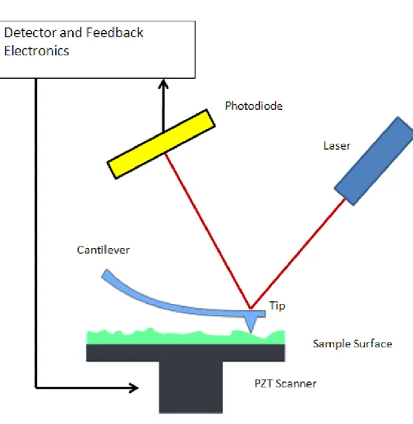
In order to simulate a tapping mode atomic force microscopy (TM-AFM) exper-iment accurately, each element of the overall system (Fig. (2.1)) should be well modelled. These elements are the (i) cantilever with a sharp tip on the free end, (ii) sample surface, (iii) interaction force between the tip and the sample surface, (iv) components of the optical lever detection scheme which is composed of a laser and a photo detector, (v) feedback control electronics.
A typical cantilever is a rectangular beam whose one end is clamped and glued to a piezoelectric actuator that drives the clamped end with a sinusoidal excita-tion. This sinusoidal excitation makes the free end of the cantilever where the
CHAPTER 2. SIMULATION BACKGROUND 5
Figure 2.1: Typical tapping mode atomic force microscopy. The elements of the system are given in the figure.
CHAPTER 2. SIMULATION BACKGROUND 6
sharp tip is located oscillate in the driving frequency with a certain amplitude. In the each cycle of the oscillation, the tip approaches to and retracts from the sample surface periodically. Due to the several interaction mechanisms (Chap-ter 2.3), there is a nonlinear in(Chap-teraction force between the tip and the sample surface. This interaction force can be attractive or repulsive according to the rel-ative position of the tip with respect to the sample surface. The tip experiences attractive forces when it is far from the sample surface, and it experiences a net repulsive force when it indents the sample surface. If the net force is attractive, the sample surface gets pulled up.
In a TM-AFM experiment, the oscillation amplitude of the cantilever is fixed to a set point amplitude during scanning. In order to achieve this, an optical lever detection scheme is used. A laser spot is reflected from the top surface of the cantilever into a photodetector matrix in the scheme. The deflection signal on the photodetector is utilized by the feedback controller electronics and the position of the sample surface relative to the cantilever base is arranged by actuating the piezo under the sample accordingly.
2.2
Torsional Harmonic Cantilever
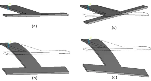
Torsional harmonic cantilever was designed in 2007 by Sahin et. al. [13] (Fig.2.2) . This cantilever is T-shaped and has a tip that is placed offset to the longitudional axis of the cantilever that creates torque on the cantilever in each tap. This torque excites the torsional modes of the cantilever. Advantage of the torsional harmonic cantilever is the ability to detect the harmonics of the tip-sample interaction force thanks to the higher resonance frequency of the first torsional mode compared to the first flexural modes. Flexural and torsional vibrations of a torsional harmonic cantilever is given in Fig.2.2 for illustration purposes.
CHAPTER 2. SIMULATION BACKGROUND 7
Figure 2.2: Vibration modes of a torsional harmonic cantilever. (a) No excitation, (b) first flexural mode is excited, (c) first torsional mode is excited, (d) first flexural and first torsional modes are both excited.
2.3
The Model
The tip-sample ensemble can be represented by a linear system with a sinusoidal excitation and a nonlinear feedback [26]. The linear system consists of multi-ple coumulti-pled harmonic oscillators each representing one vibrational mode (either flexural or torsional) of the cantilever. The nonlinear feedback is the tip-sample interaction force.
Equations of motion of each harmonic oscillator including damping are given in Eqs. (2.1) and (2.2) for ith flexural and jth torsional mode, respectively. The
variables with tilde over them represent the torsional quantities. The overall deflection of the tip (z) is defined with respect to the rest position of the surface (Fig. (2.3)). z can be calculated by the summation of the individual deflection of the each mode and the cantilever-sample distance (Xo) as given in Eq. (2.3)
CHAPTER 2. SIMULATION BACKGROUND 8 z f = flexural deflection z t = torsional deflection X
o = cantilever ï sample distance
reference direction
+ z = overall deflection z
s = surface displacement
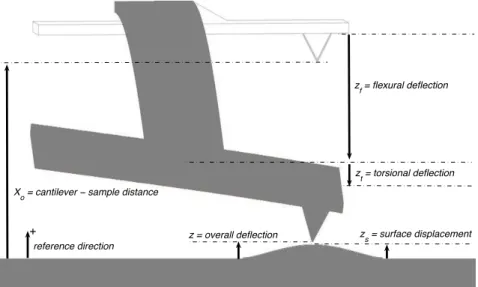
Figure 2.3: Coordinate system for the overall tip deflection of the torsional har-monic cantilever. The total deflection of the cantilever (z) on the tip side is assumed as the summation of the flexural (zf) and torsional (zt) deflections of
the cantilever. The surface displacement (zs) is included in the model. Note
that zf = !izi and zt = !jz˜j. Positive direction for the vectors of force and
deflection is depicted in the figure.
Qi, ki, fi, Fd and fd stand for the equivalent point-mass, quality factor, spring
constant, resonance frequency of ith mode of the cantilever, drive amplitude and
drive frequency, respectively. Eq. (2.4) governs the displacement of the sample surface where γs and ks represent the internal damping coefficient and spring
constant of the sample, respectively.
mi d2z i dt2 + 2πmifi Qi dzi dt + kizi = Fts(z− zs) + Fdcos(2πfdt) i = 1, 2,· · · (2.1) ˜ mj d2z˜ j dt2 + 2π ˜mjf˜j ˜ Qj d˜zj dt + ˜kjz˜j = Fts(z− zs) j = 1, 2,· · · (2.2)
CHAPTER 2. SIMULATION BACKGROUND 9 z = Xo+ " i zi+ " j ˜ zj (2.3) γs dzs dt + kszs =−Fts(z− zs) (2.4) The excitation term, Fdcos(2πfdt), is dropped in Eq. (2.2), because the
ex-citation of the torsional modes due to the drive force is negligible. Fts(z − zs)
is the single valued, displacement dependent tip-sample interaction force where zs is the displacement of the sample surface with respect to the rest position
(Fig. (2.3)). In the model, we ignore the excitation of the torsional mode due to the asymmetric mass distribution caused by the offset positioned tip.
The MDOF mechanical model of the tip-sample ensemble given above can be represented as an electrical circuit [10] as given in Fig. (2.4). By replacing the mass with an inductor, the spring with a capacitor, the damper with a resistor, displacement becomes charge and force becomes voltage. Eqs. (2.1), (2.2), (2.3) and (2.4) turn into Eqs. (2.5), (2.6), (2.7) and (2.8). Eqs. (2.5) and (2.6) cor-respond to governing equation of an RLC circuits and Eq. (2.8) corcor-responds to governing equation of an RC circuit. Qo is the corresponding charge for Xo.
Li d2q i dt2 + Ri dqi dt + qi Ci = Fts(q− qs) + A cos(2πfdt) (2.5) ˜ Lj d2q˜ j dt2 + ˜Rj d˜qj dt + ˜ qj ˜ Cj = Fts(q− qs) (2.6) q = Qo+ " i qi+ " j ˜ qj (2.7) Rs dqs dt + qs Cs =−Fts(q− qs) (2.8)
In the electrical equivalent circuit, Fts(q− qs) is a nonlinear charge controlled
CHAPTER 2. SIMULATION BACKGROUND 10
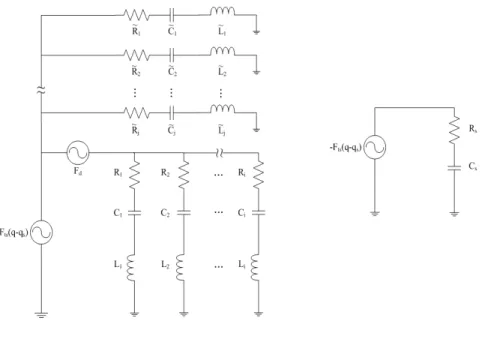
Figure 2.4: Electrical equivalent circuit of the multiple degree of freedom model of the tip-sample ensemble. The variables with tilde over them represents the torsional variables. Each of the vibrational modes is represented by a series RLC circuit where the sample surface is represented by a RC circuit.
nonlinear components that represent the loss and the stiffness of the sample, respectively. We solve Eqs. (2.5), (2.6), (2.7) and (2.8) numerically using tran-sient time domain analysis toolbox of a commercial circuit simulator1 to find the
steady-state response of the tip-sample interaction.
2.4
Tip-Sample Interaction
There are various mechanisms that constitute the tip-sample interaction such as long range interfacial forces, short range repulsive forces, adhesion, viscosity and capillary forces [27]. However, it is not a trivial task to include all the mechanisms in one simulation because of the increased numerical complexity due to lack of
CHAPTER 2. SIMULATION BACKGROUND 11
analytic expressions that relate the amount of the indentation with the force in the each mechanism of the interaction.
For the non-contact part of the oscillation cycle, we implement the long range interfacial forces which has 1/(z− zs)2 dependence. At the onset of the contact
(when z− zs= ao where ao is the interatomic distance [28]), we equate the long
range interfacial force to adhesion force predicted by DMT contact model [29] in order to maintain the continuity of the force [17].
For the contact part of the oscillation cycle, we implement a single valued, (z− zs) dependent divergent force (Fdiv) given in Eq. (2.10) that is similar to one
used in [25] to assure that z−zs ≈ ao during the indentation (Fig. 2.5). Although
the force function is single valued, because of the dissipation mechanisms included in the model, there is a hysteresis in force.
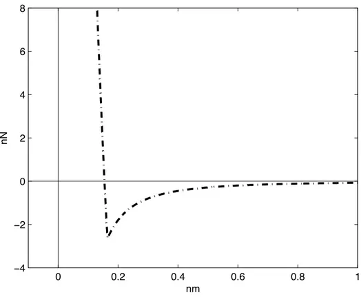
The resulting tip-sample interaction force is given in Eq. (2.9). γ, R, c stand for the surface adhesion energy, the tip radius and the unit conversion constant, respectively. Fts(z, zs) = −4πγRa2 o/(z− zs)2 z− zs > ao −4πγR + Fdiv z− zs <= ao (2.9) Fdiv = c 4 3E ∗√R(a o− z)1.15 (2.10)
The sample is modelled by a series RC circuit with a nonlinear resistance (Rs)
and a nonlinear capacitance (Cs) as given in Eq. (2.8). We use DMT contact
model to formalize the spring constant (ks) of the sample which equals to the
inverse of the capacitance (Cs) given in Eq. (2.11). E∗ stands for the effective
elastic modulus of the tip-sample ensemble. By writing Eq. (2.11), we assume that the sample has the same stiffness both in loading and unloading periods [25]. Interatomic distance (ao) is used again to maintain a finite value for Cs when
CHAPTER 2. SIMULATION BACKGROUND 12 0 0.2 0.4 0.6 0.8 1 ï4 ï2 0 2 4 6 8 nN nm
Figure 2.5: Fts vs. (z− zs). After the contact is established in the oscillation
cycle, as tip indents the surface, (z − zs) stars to shrink from ao to zero and
Fts quickly reaches the value that needed to push the surface inwards and keeps
z− zs≈ ao. Cs= 1 ks = 4 1 3E∗ & R(|zs| + ao) (2.11)
The main sources of the energy dissipation (loss) in the tip-sample interac-tion are capillary forces, hysteresis in interfacial interacinterac-tions, hysteresis in surface adhesion energy and viscoelasticity [27]. The viscous force is dependent to the de-formation and the time course of dede-formation (Eq. (2.12)) when Hertzian contact mechanics are considered. η is the viscosity of the surface. Other loss mech-anisms are modelled by a constant offset resistance (Ro) as in [25]. Thereby,
CHAPTER 2. SIMULATION BACKGROUND 13
in Eq. (2.13) in our model.
Fvis= η & R|zs| dzs dt (2.12) γs = Rs= Ro+ η & R|zs| (2.13)
2.5
Noise Analysis
There are several noise sources in the optical lever detection scheme. These are the shot noise of the photodetector, thermal mechanical noise of the cantilever, laser noise, electronic noise of the detection circuitry and mechanical vibrations of the whole system [30]. Since optical lever detection scheme is used in imaging with THC as well, all the noise sources stated above are valid for THC.
The laser noise is composed of the intensity noise, phase noise, 1/f noise and pointing noise. First three components of the laser noise are all zero in the optical lever detection [30]. The pointing noise of the laser will be neglected in the simulations. Therefore, there will be no laser dependent noise source in the model. The noise originated from the overall mechanical vibrations of the system is also neglected since the resonance frequency of the system is low compared to the cantilever.
Electronic noise is composed of the noise of the transimpedance amplifier and the Johnson noise of the feedback resistor. Resulting electrical equivalent noise circuit and the amplitude of noise sources are given in Fig. 2.6 and Table 3.3, respectively.
is is the output signal of the photodetector which is the difference of split
photodetector currents and given by is =
3πaIl
CHAPTER 2. SIMULATION BACKGROUND 14
Figure 2.6: Equivalent noise circuit of the system consists of the photodetector, the cantilever and the transimpedance amplifier. is, ish, im, en, in, eR represent
the sources corresponding to the output signal of the photodetector, shot noise of the photodetector, thermomechanical noise of the cantilever, input noise volt-age of the transimpedance amplifier, input noise current of the transimpedance amplifier and Johnson noise voltage of the transimpedance amplifier, respectively.
CHAPTER 2. SIMULATION BACKGROUND 15
where ξ stands for the deflection of the tip. The total mean square shot noise current of the photodetector is given by
< i2sh >= 2qBIl (2.15)
where q, B are the elementary electronic charge and the detection bandwidth, respectively. Mean square deflection of the thermally excited cantilever and the corresponding mean square current on photodetector for each mode is given in Eq. (2.16). < ξn2 >= 4KT B Qikiwi , < i2m >= 3πaIl 2λl < ξ 2 n > (2.16)
The mean square input noise voltage and current of the transimpedance am-plifier are < e2
n>, < i2n> and these depend on the amplifier characteristics. The
mean square voltage of Johnson noise is given by
< e2R>= 4KT BR (2.17)
where R is the resistance of the resistor. In Table 3.3, the parameters of the first three flexural modes and the first torsional mode of the cantilever are given. The dimensions of the cantilever are also given in Table 3.3 (subscript ’t’ stands for torsional).
The torsional vibrations are below the noise level of the photodetector with the given noise sources in Table 3.3. Therefore, the detection bandwidth should be decreased somehow to measure the torsional harmonics. Lock-in amplifiers can be used, however one can receive only one harmonic with one lock-in am-plifier which is impractical. In order to decrease the detection bandwidth, time-averaging is preferred in experimental studies assuming the vibration signal is quasi-periodic [13]. We model the effect of the time-averaging by downscaling the rms values of the noise sources by √N , where N is the number of the oscil-lation cycles used in averaging.
CHAPTER 2. SIMULATION BACKGROUND 16
2.6
Implementation of the Overall System as an
Electrical Circuit
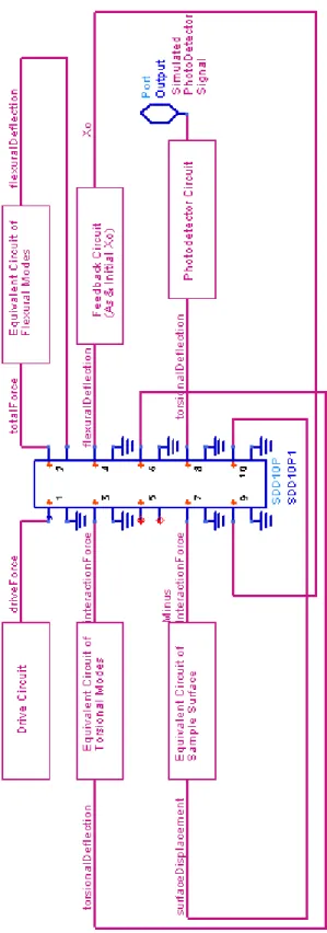
The overall system is modelled as an electrical circuit that is composed of the drive circuit, equivalent circuit of the first three flexural modes, equivalent circuit of the first torsional mode, equivalent circuit of the sample surface, feedback circuit and the photodetection circuit. The input/output relation of these circuits are given in Fig. 2.7.
CHAPTER 2. SIMULATION BACKGROUND 17
CHAPTER 2. SIMULATION BACKGROUND 18
2.6.1
Drive Circuit
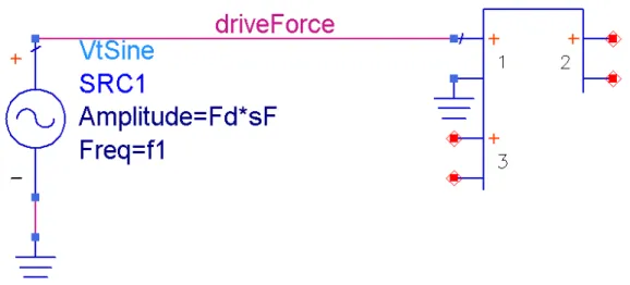
The drive circuit is used to generate a simple sinusoidal excitation in the resonance frequency of the first flexural mode of the cantilever. The related parameters are the amplitude of the excitation (Fd), drive frequency (f1) and a scaling factor (sf).
The typical order of the force and deflections are in nN and nm, respectively, which are quite small orders for a simulation engine to deal with. Therefore, a scaling factor (sf) is used to relax the simulation engine. The values of the
parameters of the cantilever are also scaled by sF accordingly in order not to
alter the results. Ability to use a scaling factor like sf is a result of the linear
transfer function of the cantilever in each mode.
Figure 2.8: Circuit that is used to drive the cantilever in its first flexural resonant mode.
CHAPTER 2. SIMULATION BACKGROUND 19
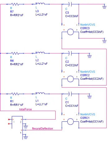
2.6.2
Equivalent Circuit of the First Three Flexural
Modes of the Cantilever
The total force is the summation of the tip-sample interaction force and the drive force in time. Each mode is driven by the total force. The deflection of the each mode is the charge on the corresponding capacitor. The overall flexural deflection is the summation of the deflection of the each mode in time.
CHAPTER 2. SIMULATION BACKGROUND 20
2.6.3
Equivalent Circuit of the First Torsional Mode of
the Cantilever
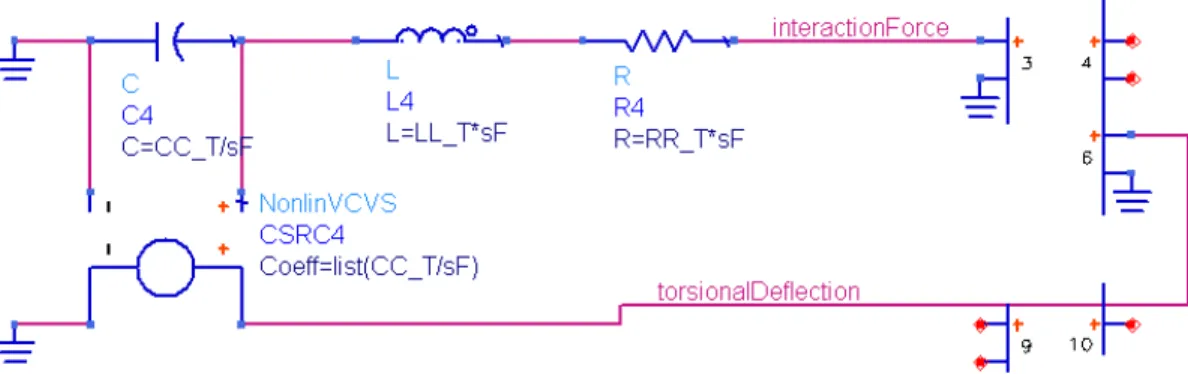
The torsional mode is driven by the tip-sample interaction force only. The tor-sional deflection is read from the charge on the capacitor.
CHAPTER 2. SIMULATION BACKGROUND 21
2.6.4
Equivalent Circuit of the Sample Surface
The sample surface is subjected to the minus of the tip-sample interaction force. The surface is modelled by a resistor with nonlinear resistance (Rs) and a
capac-itor with nonlinear capacitance (Cs) in series. The capacitor is implemented in
the fifth port of the SDD6P1 box. In order to relax the simulation engine some interval variables are used.
CHAPTER 2. SIMULATION BACKGROUND 22
2.6.5
Feedback Circuit
In order to achieve a given set point amplitude (As), we used a
proportional-integral (PI) controller. Thereby, the value of Xo (Fig. 2.3) that is required to
achieve the desired As is found from an arbitrary initial value of Xo. Magnitude
of the first flexural harmonic is compared with the set point amplitude As. The
error is integrated, multiplied by a gain factor and the difference signal is added to the initial value of Xo.
CHAPTER 2. SIMULATION BACKGROUND 23
2.6.6
Photodetector Circuit
The noisy deflection signal is first amplified by the internal conversion gain of the photodetector, then amplified by the transimpedance amplifier. The equivalent noise sources are also added to the circuit.
Chapter 3
SIMULATION RESULTS
This chapter begins with the presentation of the effect of the enhanced higher order vibrations on the steady-state dynamics of the tapping mode atomic force microscopy (TM-AFM) where noise is not included. After that, the chapter continues with the presentation of the material characterization with the torsional harmonic cantilevers in the presence of noise.
3.1
Effect of the Enhanced Higher Order
Vibra-tions on Steady-State Dynamics
The imaging conditions and the parameters of the torsional harmonic cantilever used in the simulations are the same with those used in [3] and given in Table 3.1. The sample parameters and the steady state values of some simulation outputs for two different samples are given in Table 3.2. The sample parameters are chosen similar to those used in [6, 27, 31]. We assume that the surface adhesion energy (γ) and the remaining loss mechanisms other than viscosity are same for both samples which concludes that the offset loss component (Ro) is same for
both samples (Eq. 2.13). The calculated tip trajectory, surface displacement,
CHAPTER 3. SIMULATION RESULTS 25
Table 3.1: Cantilever parameters and imaging conditions
Parameter Symbol Unit Value
resonance frequency f1 kHz 55 f2 344 f3 965 ft 905 spring constant k1 N/m 2.6 k2 102 k3 800 kt 500 quality factor Q1 100 Q2 250 Q3 450 Qt 800 tip radius R nm 7 drive frequency fd kHz 55 free-air amplitude Ao nm 38 set-point amplitude As 31
Table 3.2: Sample parameters and values of some parameters at steady state
Compliant Sample Stiff Sample
Parameter Symbol Unit Value Value
effective elastic modulus E∗ GP a 0.1 1
surface adhesion energy γ mJ/m2 30 30
viscosity η P a· s 30 800
offset loss coefficient Ro nΩ 50 50
maximum deformation δ nm 2.8 0.66
cantilever-sample distance Xo nm 28.3 30.4
maximum torsional deflection A˜ pm 11.7 22.9
peak repulsive force Fts,peak nN 3.3 6.9
CHAPTER 3. SIMULATION RESULTS 26
torsional vibrations, torsional harmonics up to torsional resonance and the tip-sample interaction during indentation process are given in Figs. 3.1, 3.2, 3.3 and 3.4, respectively, for two different samples. One sample is compliant (100 MPa) where the other is stiff (1 GPa).
Well known characteristics of the TM-AFM are also observed and verified in the simulations. The tip trajectory is almost sinusoidal since the vibration am-plitude of the higher order flexural modes and the fundamental torsional mode is three orders of magnitude smaller than that of the first flexural mode which means torsional vibrations do not disturb the tapping mode operation [32]. The hysteresis in the surface elongation between loading and unloading periods (de-picted by star in Fig. 3.1) is observed since there is a certain amount of energy coupled to the surface in each cycle. This is more pronounced in the compliant sample case. It is observed that the contact time and the maximum deforma-tion decrease with the sample stiffness where the maximum repulsive interacdeforma-tion force increases. Although these observations are common facts of TM-AFM, the agreement of theory with our model is important for the validity of the new implications of the simulation results.
The torsional vibrations, which is the main scope of this work, are a little bit complicated in shape and depends on the tip-sample interaction force which depends on the sample parameters indeed (Fig. 3.2). There is a slowly decaying torsional oscillation remaining from the preceding tap before contact due to the high quality factor of the torsional mode. With the impact of the tip to the sam-ple, oscillations get complex in shape due to the excitation of the torsional mode by the nonlinear tip-sample interaction force. There is a certain DC torsional deflection on the cantilever during indentation period because the tip acts like a pivot point for the cantilever to bend. There is a hysteresis in the amplitude of torsional vibrations between loading and unloading time instants because of the hysteresis in the tip-sample interaction force. This effect is more pronounced in the compliant sample case. After the contact, the cantilever oscillates in the torsional resonance with a slow decay until the next tap.
CHAPTER 3. SIMULATION RESULTS 27 5.394 5.395 5.396 5.397 5.398 5.399 5.4 5.401 5.402 5.403 ï3 ï2 ï1 0 1 2 3 ms nm 5.394 5.395 5.396 5.397 5.398 5.399 5.4 5.401 5.402 5.403 ï3 ï2 ï1 0 1 2 3 ms nm z zs z zs
*
a) b)Figure 3.1: Tip displacement and surface motion in the case of (a) compliant and (b) stiff sample after three Q1 cycles. Note that z−zs is always greater than zero.
There is a hysteresis in the surface elongation (depicted by star on the figure) because of energy dissipation.
CHAPTER 3. SIMULATION RESULTS 28 5.394 5.395 5.396 5.397 5.398 5.399 5.4 5.401 5.402 5.403 ï10 ï5 0 5 10 15 20 25 ms pm 5.394 5.395 5.396 5.397 5.398 5.399 5.4 5.401 5.402 5.403 ï10 ï5 0 5 10 15 20 25 ms pm a) b)
Figure 3.2: Torsional vibrations on the torsional harmonic cantilever in the case of (a) compliant and (b) stiff sample after three Q1 cycles.
CHAPTER 3. SIMULATION RESULTS 29 0 200 400 600 800 1000 1200 0 0.2 0.4 0.6 0.8 1 kHz pm 0 200 400 600 800 1000 1200 0 1 2 3 4 5 6 7 kHz pm a) b)
*
Figure 3.3: Harmonics of the torsional vibrations up to the resonance of the torsional mode in the case of (a) compliant and (b) stiff sample after three Q1 cycles. Axis limit of y-coordinate is not preserved because of illustration purposes. Star is used to depict the first zero crossing of the magnitude of the harmonics.
CHAPTER 3. SIMULATION RESULTS 30 5.396 5.397 5.398 5.399 5.4 5.401 ï2 0 2 4 6 8 ms nN 5.396 5.397 5.398 5.399 5.4 5.401 ï2 0 2 4 6 8 ms nN actual recovered actual recovered a) b)
Figure 3.4: Actual tip-sample interaction force and recovered one from first 16 torsional harmonics in the case of (a) compliant and (b) stiff sample after three Q1 cycles.
CHAPTER 3. SIMULATION RESULTS 31
The peak amplitude of the torsional deflection and the amplitude of non-contact oscillation is higher for the stiff sample. It is observed that the non-contact time can be deduced from the torsional vibrations and it exhibits a stiffness contrast between materials just as in the case of tip-sample interaction force. The difference between amplitude of before and after contact oscillations is small in stiff sample case where it is large in compliant sample case. The amplitude difference is just the result of decay of the high-Q torsional mode in stiff sample case. However, in the compliant sample case, besides simple mode decay, the tip-sample interaction enhances the oscillation close to the torsional resonance at one tap and then reduces it in the next tap as a result of the phase difference between the oscillation on the cantilever and the harmonic of tip-sample interaction force close to the torsional resonance.
The frequency spectrum of the torsional vibrations changes with sample stiff-ness (Figure 3.3)). In the case of the stiff sample, the spectrum of the torsional vibrations is more flat up to the torsional resonance. This can be explained by remembering two facts (i) the spectrum of the torsional vibrations is simply the product of the spectrum of the tip-sample interaction force and the transfer func-tion of the torsional mode, (ii) the spectrum of the tip-sample interacfunc-tion force flattens (the first zero crossing of the magnitude of the harmonics (depicted by the star in Fig. 3.3)) moves to the higher frequencies) as sample gets stiffer under the same imaging conditions [12]. The peak around 900 kHz in the magnitude spectrum is due to the peak amplification of the torsional mode, that is, due to torsional resonance.
There are 16 torsional harmonics up to the torsional resonance. These har-monics are the scaled version of the harhar-monics of the tip-sample interaction by 1/kt where kt is the spring constant of the torsional mode. The harmonics of the
tip-sample interaction force placed after the torsional resonance are subjected to the high attenuation of the torsional mode. The magnitude of these torsional harmonics are near the noise level. Using first 16 torsional harmonics, one can recover the tip-sample interaction force in time [13, 33] and estimate the material properties [3].
CHAPTER 3. SIMULATION RESULTS 32 108 109 0 0.2 0.4 0.6 0.8 1 1.2 1.4 1.6 1.8 E* pm 6th 8th 10th 12th 14th
Figure 3.5: Change in magnitude of various harmonics of the torsional vibrations with respect to the effective elastic modulus
The recovered tip-sample interaction force curve using first 16 torsional har-monics overlaps with the actual tip-sample interaction force in the compliant sample case where it slightly deviates in the stiff sample case (Fig. 3.4). We used the algorithm proposed in [13] in order to estimate the effective elastic modulus using the recovered tip-sample interaction force curve. The estimated effective elastic modulus (E∗) values are 107 MPa and 1.4 GPa for the compliant and the
stiff sample, respectively. Although noise is not included in the model, there is an error in the estimation. This error is a result of the (i) reconstruction of the tip-sample interaction force with a finite number of harmonics and (ii) ignoring the interactions in contact other that the ones proposed by DMT model in the estimation algorithm.
CHAPTER 3. SIMULATION RESULTS 33
We plotted the magnitude of the torsional harmonics while scanning the sam-ple stiffness values between the compliant and the stiff one (Figure 3.5) where the surface energy and the imaging parameters are kept constant (γ = 30mJ/m2).
The monotonically increasing part of the curve is the range where a particular harmonic is sensitive to the change in elastic modulus. For example, one can use 8th torsional harmonic to get material contrast between the samples with elastic
modulus starting from 0.1 GPa. Moreover, 24th harmonic is more sensitive
com-pared to the lower harmonics for the samples with elastic modulus greater than 300 MPa. In short, the higher harmonics are more sensitive to the elasticity than the lower harmonics and the range where a harmonic is sensitive corresponds a stiffer range when the harmonic number increases. Thereby, it is convenient to use the lower harmonics for compliant samples and the higher harmonics for stiff samples.
These results confirm that the torsional harmonic cantilever is capable of re-ceiving sufficient number of higher harmonics of the tip-sample interaction with a tolerable attenuation to estimate material properties in a certain range of ma-terials without disturbing the tapping mode operation.
3.2
Material Characterization with the
Tor-sional Harmonic Cantilevers in the Presence
of Noise
For the imaging conditions (fd, Ao, As) given in Table 3.3, the simulated torsional
signal is given in Fig 3.6a. The torsional signal is Fourier transformed, multiplied by the inverse of the transfer function of the torsional mode of the cantilever and the harmonics other than the first M are filtered. Resulting spectrum is inverse Fourier transformed. Recovered tip-sample interaction force (TSIF) with M=15 and actual TSIF is given in Fig 3.6b. E∗ is estimated as 98.5 MPa by curve
fitting to repulsive part of TSIF between peak force and %20 of it, where actual E∗ is 100 MPa.
CHAPTER 3. SIMULATION RESULTS 34
Table 3.3: Simulation Parameters Cantilever resonance frequency f1 kHz 55 f2 344.3 f3 965.3 ft 905 spring constant k1 N/m 2.6 k2 101.8 k3 800.8 kt 500 quality factor Q1 —- 100 Q2 250 Q3 450 Qt 800 length l µm 300 width of base − 30
width of free end − 55
thickness − 4.5
tip offset − 25
tip radius $ nm 7
Noise Sources
shot noise current < ish> pA/
√
Hz 12.65
input noise current < in > 2
input noise voltage < en > nV /
√
Hz 20
Johnson noise voltage (R=1M ) < eR > 17.89
PD Current
Laser spot size a µm 30
Laser wavelength λ nm 670 Responsivity of photodetector R1 —- 0.5 Reflectivity of cantilever R2 —- 1 Power of laser P mW 1 Imaging Conditions Drive frequency fd kHz 55 Free-air amplitude Ao nm 38
CHAPTER 3. SIMULATION RESULTS 35
The same analysis is done for a wide range of materials from 10 MPa to 10 GPa and the estimated values of E∗ are given in Fig. 3.7. The stiff samples are
under-estimated whereas the compliant samples are overunder-estimated for M=15 (circles in Fig. 3.7). This result is in perfect agreement with experimental results [32].
The harmonics after the first zero crossing of the spectrum of TSIF (Fig. 3.6c) do not include much information about the slope of the repulsive part of TSIF and increase the effect of the noise if they are used in recovery. Therefore, we propose to use the harmonics up to the first zero crossing in the recovery instead of the first M. Thereby the accuracy of estimation is improved (stars in Fig. 3.7). The portion of the repulsive part of TSIF that is used in the curve fitting affects the estimation. Since a finite number of torsional harmonics can be de-tectable and used in the recovery of TSIF, the slope of the repulsive part of TSIF can have different values for different portions. Since an accurate estimation over a wide range of materials is desired, there is not an optimum portion of TSIF that curve fitting will be done.
CHAPTER 3. SIMULATION RESULTS 36 3.572 3.574 3.576 3.578 3.58 3.582 3.584 3.586 3.588 ï0.02 0 0.02 0.04 0.06 V 3.572 3.574 3.576 3.578 3.58 3.582 3.584 3.586 3.588 ï3 ï2 ï1 0 1 2 3 4 ms nN recovered actual 0 2 4 6 8 10 12 14 16 18 0 0.1 0.2 0.3 0.4 Harmonic Number nN recovered actual a) b) c)
Figure 3.6: Simulation outcomes for a sample with E∗=100MPa a) noisy pho-todetector signal (N=50) b) recovered TSIF (M=15), estimated E∗ is 98.495MPa
CHAPTER 3. SIMULATION RESULTS 37 107 108 109 1010 107 108 109 1010 Actual E* (Pa) Estimated E * (Pa)
Figure 3.7: Estimations over a wide range of materials in the presence of noise. Estimations with M=15 are depicted by circles. Estimations that the harmonics up to the first zero crossing of the spectrum of TSIF is used are depicted by dots.
Chapter 4
CONCLUSIONS
The multiple degree of freedom model of the tip-sample ensemble including the fundamental torsional mode and the first three flexural modes is realized. Thereby, the steady-state response of the torsional harmonic cantilever is sim-ulated. General characteristics and material dependency of the torsional vibra-tions on a torsional harmonic cantilever is investigated. It is observed that the torsional vibrations on a torsional harmonic cantilever are three orders of mag-nitude smaller than the overall flexural vibrations which means they do not alter tapping mode operation.
Since the torsional mode is excited by the tip-sample interaction force only, the spectrum of the torsional vibrations is just the scaled version of the spectrum of the tip-sample interaction with the transfer function of the torsional mode. Therefore, there is a one-to-one correspondence between the tip-sample inter-action force and the torsional vibrations. It is demonstrated that the torsional harmonics up to the torsional resonance are sufficient to estimate the elasticity of a sample with tolerable error for a certain range of elasticity. Thereby, it is verified that the torsional harmonic cantilever is capable of material property mapping.
The variation of the torsional harmonics on a torsional harmonic cantilever with sample stiffness is simulated. It is shown that the sensitivity of a particular
CHAPTER 4. CONCLUSIONS 39
torsional harmonic changes with sample stiffness. As the sample gets stiffer, the sensitivity of a particular torsional harmonic decreases. Moreover, for a given range of stiffness values, the higher harmonics of the torsional vibrations are more sensitive to change in stiffness rather than the lower harmonics.
A nonlinear model of the sample surface is realized. The stiffness of a sample is modelled with a nonlinear spring and damping of the surface is modelled with a nonlinear damper. A nonlinear modelling of the surface is required to obtain more realistic results for the tip-sample interaction and the energy dissipation. We believe that this work will motivate others who want to utilize more realistic surface models.
A noise analysis of the overall system is performed and the noise sources are added to the model. The noisy torsional vibration signal on photodetector is simulated. The tip-sample interaction force is recovered from the harmonics of the torsional signal and the estimation of effective elastic modulus (E∗) of the
sample is achieved. The same analysis is done for a wide range of materials. It is demonstrated that the torsional harmonic cantilevers are capable of es-timating material properties over a wide range of materials. The number of the torsional harmonics used in the recovery of the tip-sample interaction force and the portion of the repulsive part of the tip-sample interaction force that is used in the curve fitting affect the estimation accuracy. It is observed that with a fixed number of harmonics used in the recovery of TSIF and with the curve fitting algorithm, stiff side of the material spectrum is underestimated where compliant side is overestimated. It is also observed that the harmonics higher than the first zero crossing frequency of the spectrum of TSIF does not affect the slope of the tip-sample interaction force much. Therefore, it is beneficial to use the first harmonics up to the first zero crossing in the estimation of E∗ in order to get rid
Bibliography
[1] G. Binnig, C. F. Quate, and C. Gerber, “Atomic force microscope,” Phys. Rev. Lett., vol. 56, pp. 930–933, 1986.
[2] Q. Zhong, D. Inniss, K. Kjoller, and V. B. Elings, “Fractured polymer/silica fiber surface studied by tapping mode atomic force microscopy,” Surf. Sci., vol. 290, pp. L688–L692, 1993.
[3] O. Sahin and N. Erina, “High-resolution and large dynamic range nanome-chanical mapping in tapping-mode atomic force microscopy,” Nanotechnol-ogy, vol. 19, pp. 445 717–445 725, 2008.
[4] D. Klinov and S. Magonov, “True molecular resolution in tapping-mode atomic force microscopy with high-resolution probes,” Appl. Phys. Lett., vol. 84, pp. 2697–2699, 2004.
[5] J. P. Cleveland, B. Anczykowski, A. E. Schmid, and V. B. Elings, “Energy dissipation in tapping-mode atomic force microscopy,” Appl. Phys. Lett., vol. 72, pp. 2613–2615, 1998.
[6] A. SanPaulo and R. Garcia, “Unifying theory of tapping-mode atomic-force microscopy,” Phys. Rev. B, vol. 66, pp. 41 406–41 409, 2002.
[7] R. W. Stark and W. M. Heckl, “Fourier transformed atomic force microscopy: tapping mode atomic force microscopy beyond the hookian approximation,” Surf. Sci., vol. 457, pp. 219–228, 2000.
BIBLIOGRAPHY 41
[8] M. Stark, R. W. Stark, W. M. Heckl, and R. Guckenberger, “Spectroscopy of the anharmonic cantilever oscillations in tapping-mode atomic-force mi-croscopy,” Appl. Phys.Lett., vol. 77, pp. 3293–3295, 2000.
[9] R. Hillenbrand, M. Stark, and R. Guckenberger, “Higher-harmonics gener-ation in tapping-mode atomic-force microscopy:insights into the tipsample interaction,” Appl. Phys. Lett., vol. 76, pp. 3478–3480, 2000.
[10] O. Sahin and A. Atalar, “Simulation of higher harmonics generation in tapping-mode atomic force microscopy,” Appl. Phys. Lett., vol. 79, pp. 4455– 4457, 2001.
[11] T. R. Rodriguez and R. Garcia, “Tip motion in amplitude modulation tapping-mode atomic-force microscopy: Comparison between continuous and point-mass models,” Appl. Phys. Lett., vol. 80, pp. 1646–1648, 2002.
[12] O. Sahin, G. Yaralioglu, R. Grow, S. F. Zappe, A. Atalar, C. Quate, and O. Solgaard, “High-resolution imaging of elastic properties using harmonic cantilevers,” Sensors and Actuators A, vol. 114, pp. 183–190, 2004.
[13] O. Sahin, S. Magonov, C. Su, C. F. Quate, and O. Solgaard, “An atomic force microscope tip designed to measure time-varying nanomechanical forces,” Nature Nanotechnology, vol. 2, pp. 507–514, 2007.
[14] H. Li, Y. Chen, and L. Dai, “Concentrated-mass cantilever enhances multi-ple harmonics in tapping-mode atomic force microscopy,” Appl. Phys. Lett., vol. 92, pp. 151 903–151 905, 2008.
[15] A. F. Sarioglu and O. Solgaard, “Cantilevers with integrated sensor for time-resolved force measurement in tapping-mode atomic force microscopy,” Appl. Phys. Lett., vol. 93, pp. 23 114–23 116, 2008.
[16] A. G. Onaran, M. Balantekin, W. Lee, W. L. Hughes, B. A. Buchine, R. O. Guldiken, Z. Parlak, C. F. Quate, and F. L. Degertekin, “A new atomic force microscope probe with force sensing integrated readout and active tip,” Rev. Sci. Instrum., vol. 77, pp. 23 501–23 507, 2006.
BIBLIOGRAPHY 42
[17] M. Balantekin, A. G. Onaran, and F. L. Degertekin, “Quantitative mechan-ical characterization of materials at the nanoscale through direct measure-ment of time-resolved tipsample interaction forces,” Nanotechnology, vol. 19, pp. 85 704–85 709, 2008.
[18] T. R. Rodriguez and R. Garcia, “Compositional mapping of surfaces in atomic force microscopy by excitation of the second normal mode of the microcantilever,” Appl. Phys. Lett., vol. 84, pp. 449–451, 2004.
[19] N. F. Martinez, S. Patil, J. R. Lozano, and R. Garcia, “Enhanced compo-sitional sensitivity in atomic force microscopy by the excitation of the first two flexural modes,” Appl. Phys. Lett., vol. 89, pp. 153 115–153 117, 2006. [20] R. Proksch, “Multifrequency, repulsive-mode amplitude-modulated atomic
force microscopy,” Appl. Phys. Lett., vol. 89, pp. 113 121–113 123, 2006. [21] R. W. Stark, N. Naujoks, and A. Stemmer, “Multifrequency electrostatic
force microscopy in the repulsive regime,” Nanotechnology, vol. 18, pp. 65 502–65 508, 2007.
[22] U. Bostanci, M. K. Abak, O. Aktas, and A. Dana, “Nanoscale charging hysteresis measurement by multifrequency electrostatic force spectroscopy,” Appl. Phys. Lett., vol. 92, pp. 93 108–93 110, 2008.
[23] M. K. Abak, O. Aktas, R. Mammadov, I. Gurel, and A. Dana, “Parametri-cally coupled multiharmonic force imaging,” Appl. Phys. Lett., vol. 92, pp. 223 113–223 115, 2008.
[24] D. Platz, E. A. Tholen, D. Pesen, and D. B. Haviland, “Intermodulation atomic force microscopy,” Appl. Phys. Lett., vol. 92, pp. 153 106–153 108, 2008.
[25] O. Sahin and A. Atalar, “Analysis of tip-sample interaction in tapping-mode atomic force microscope using an electrical circuit simulator,” Appl. Phys. Lett., vol. 78, pp. 2973–2975, 2001.
BIBLIOGRAPHY 43
[26] M. Stark, R. W. Stark, W. M. Heckl, and R. Guckenberger, “Inverting dy-namic force microscopy: From signals to time-resolved interaction forces,” Proc. Natl Acad. Sci. USA, vol. 99, pp. 8473–8478, 2002.
[27] R. Garcia, C. J. Gomez, N. F. Martinez, S. Patil, C. Dietz, and R. Magerle, “Identification of nanoscale dissipation processes by dynamic atomic force microscopy,” Physical Review Letters, vol. 97, p. 016103, 2006.
[28] R. Garcia and A. SanPaulo, “Dynamics of a vibrating tip near or in inter-mittent contact with a surface,” Phys. Rev. B, vol. 61, pp. R13 381–R13 384, 2000.
[29] J. N. Israelachvili, Intermolecular and Surface Forces. London: Academic, 1992.
[30] G. G. Yaralioglu, A. Atalar, S. Manalis, and C. F. Quate, “Analysis and design of an interdigital cantilever as a displacement sensor,” J. Appl. Phys., vol. 83, pp. 7405–7415, 1998.
[31] J. Tamayo and R. Garcia, “Effects of elastic and inelastic interactions on phase contrast images in tapping-mode scanning force microscopy,” Appl. Phys. Lett., vol. 71, pp. 2394–2396, 1997.
[32] O. Sahin and N. Erina, “High-resolution and large dynamic range nanome-chanical mapping in tapping-mode atomic force microscopy,” Nanotechnol-ogy, vol. 19, pp. 445 717–445 725, 2008.
[33] O. Sahin, “Harnessing bifurcations in tapping-mode atomic force microscopy to calibrate time-varying tip-sample force measurements,” Review of Scien-tific Instruments, vol. 78, p. 103707, 2007.