Human activity classification with miniature inertial and magnetic sensor signals

HUMAN ACTIVITY CLASSIFICATION WITH MINIATURE INERTIAL AND

MAGNETIC SENSOR SIGNALS

Murat Cihan Y¨uksek and Billur Barshan

Bilkent University, 06800 Ankara, Turkey

tel: (90-312) 290-2384, (90-312) 290-2161, fax: (90-312) 266-4192, e-mail: {yuksek, billur}@ee.bilkent.edu.tr url: www.ee.bilkent.edu.tr

ABSTRACT

This study provides a comparative performance assessment of var-ious pattern recognition techniques on classifying human activities that are performed while wearing miniature inertial and magnetic sensors. Activities are classified using five sensor units worn on the chest, the arms, and the legs. Each sensor unit comprises a tri-axial accelerometer, a tri-axial gyroscope, and a tri-axial magnetome-ter. The classification techniques compared in this study are: naive Bayesian (NB), artificial neural networks (ANN), dissimilarity-based classifier (DBC), various decision-tree algorithms, Gaussian mixture model (GMM), and support vector machines (SVM). The methods that result in the highest correct differentiation rates are found to be GMM (99.1%), ANN (99.0%), and SVM (98.9%).

1. INTRODUCTION

Human activity recognition has received considerable interest re-cently because of its potential applications in a wide range of fields such as biomechanics, ergonomics, remote monitoring of physically or mentally disabled, elderly, and children, detecting and classifying falls, medical diagnosis and treatment, home-based rehabilitation, animation and film making, computer games, professional simula-tors, and virtual reality. Despite the fact that most studies have em-ployed computer vision for this purpose, use of miniature inertial sensors such as accelerometers and gyroscopes has certain advan-tages [1]. These sensors are capable of providing dynamic motion information through direct measurements in 3-D. Processing 1-D signals acquired with these sensors is much simpler compared to dealing with multiple camera projections and occlusions. In some studies, inertial sensors are used in conjunction with magnetome-ters [2].

Earlier work on body-worn inertial sensor based activity recog-nition is fragmented, of limited extent, and mostly unsystematic in nature. Due to the lack of a common ground among differ-ent researchers, results published so far are difficult to compare, synthesize, and build upon in a manner that allows broad conclu-sions to be reached. Previous studies focus on classifying sitting, lying, and standing [3], as these postures are relatively easy to dis-tinguish using the static component of acceleration. Disdis-tinguishing between walking and ascending/descending stairs has also been per-formed [4]. The signal processing and motion detection techniques employed, and the configuration, number, and type of sensors differ widely among the studies, from using a single accelerometer [5] to as many as 12 [6] on different parts of the body. To the best of our knowledge, guidance on finding a suitable configuration, number, and type of sensors does not exist [4].

In this study, several classification methods are tested on 19 different daily and sports activities using the data acquired from in-ertial sensors and magnetometers worn on five different parts of the body. Various features are extracted from the raw sensor signals and an unsupervised feature transformation method is used that maps the original feature space to another feature space where the most informative features can be determined. The classification tests are performed systematically considering all possible combinations of

sensor types and sensor locations on the body. The results are evalu-ated in terms of correct classification rates and computational costs.

2. CLASSIFICATION TECHNIQUES

Brief descriptions of the classification techniques used in this study are given in this section. More details can be found in [7]. The algorithms for these techniques are provided on two commonly used open source environments: WEKA, a Java-based software [8]; and PRTools, a MATLAB toolbox [9]. We associate a class wiwith each activity type (i = 1, . . . , c). Every feature vector x = [x1, x2, . . . , xN]T in the set of training patterns X = {x1, x2, . . . , xI} is labeled with corresponding class wiif it falls in the region Ωi, i = 1, . . . , c. A rule that partitions the decision space into regions Ωj is called a decision rule. Each one of these regions corresponds to a different activity type.

2.1 Naive Bayesian (NB)

Naive Bayes classifier is based on the Bayes’ theorem and calculates the posterior probabilities according to the probabilistic models of each class. In this method, the probability density function is mod-eled as a normal distribution whose parameters (mean and variance) are estimated by maximum likelihood estimation. A simplifying as-sumption in the NB method is that the features are considered to be independent of each other and the model parameters are calculated accordingly. Classification is made based on maximum a posteriori (MAP) decision rule with equal priors initialized once the posterior probabilities are calculated.

2.2 Artificial Neural Networks (ANN)

A two-layer ANN is considered for classifying human activities. The input layer has N = 30 neurons, equal to the reduced dimen-sion of the feature vectors and the output layer has c = 19 neu-rons, equal to the number of classes. The sigmoid function, used as the activation function in the input and output layers, is given by h(x) = (1 + e−x)−1. The neurons in the ANN are trained with the back-propagation algorithm which is based on the least mean squares method and the gradient-descent algorithm. The learning and momentum constants of the back-propagation algorithm are both selected as 0.05.

2.3 Dissimilarity Based Classifier (DBC)

In this method, a classifier based on Fisher linear discriminant anal-ysis (FLDA) is found using the data that is a dissimilarity mapping of the original feature vectors. A dissimilarity mapping is defined to be F(·, R) : X → Rr_{from X to the so called dissimilarity space.} The r-element set R is called the representation set and consists of feature vectors so that it can be any subset of X . Using the vectors in the dissimilarity space, c − 1 classifiers are built based on FLDA to perform the classification in c-dimensional space. The notion of dissimilarity spacein which objects are characterized by relation to other objects instead of features or models is a recent concept in pattern recognition. In this study, the feature vectors in X are treated as objects and the vectors in R are chosen randomly with r = 100.

2.4 Decision-Tree Methods

2.4.1 Trees Using J48 Algorithm (J48-T)

J48 method implements the C4.5 algorithm for generating a pruned or an unpruned C4.5 decision-tree learner which is an improved version of the ID3 learner. Both ID3 and C4.5 algorithms are de-veloped by Ross Quinlan. J48 builds decision trees from a set of labeled training data using the concept of normalized information gain. This concept is a splitting criterion that is used for selecting the feature that most effectively splits the given set of feature vec-tors at a tree node.

2.4.2 Naive Bayes Trees (NB-T)

NB-T is a hybrid classifier that combines principles governing NB classifier and decision-tree notion. The hybrid algorithm is similar to the classical recursive decision-tree partitioning schemes, except that the leaf nodes created are NB classifiers instead of nodes pre-dicting a single class. The main drawback of this method is that if the assumptions regarding the independence of features fail, perfor-mance cannot be improved by increasing the size of the data set. 2.4.3 Random Forest (RF-T)

Random forests are a combination of tree predictors such that each tree depends on the values of a random vector sampled indepen-dently and with the same distribution for all trees in the forest. The forest is constructed using the bagging method along with random feature selection at a node. The rule at each node is determined us-ing normalized information gain similar to J48 algorithm. Once the trees are constructed, each tree casts a unit vote for the most pop-ular class at a given input. The parameters for this method are the number of random features to select from at a node and the number of trees in the forest. These are set to 5 and 10, respectively. 2.5 Gaussian Mixture Model (GMM)

In GMM classifier, each feature vector in the training set is assumed to be associated with a mixture of m different and independent multi-variate normal distributions. Each distribution has a probabil-ity densprobabil-ity function pj(xi| µj, Σj) where µjand Σjare the mean vector and the covariance matrix of the jth mixture component, re-spectively. The distribution of the model is expressed as:

p(xi| Θ) = m

∑

αjpj(xi| θj) (1) where Θ = (α1, . . . , αm; θ1, . . . , θm) such that αj ≥ 0 and ∑m_j=1αj= 1. Here, an analytical expression for θjcan be obtained for the special case of GMM for which θj= (µj,Σj). There are five different expressions to initialize the training. The expression for the arbitrary covariance matrix and the corresponding mean vector is used in this study. Then, the Expectation-Maximization (EM) al-gorithm is implemented to estimate Θ. The model is evaluated for different cases where the number of mixtures in the model varies from one to four.

2.6 Support Vector Machines (SVM)

In SVM classification technique, it is desired to estimate a function f : R → {±1} to label the training feature vectors with −1 and +1. Here, the problem is posed as a binary classification problem. Assuming there are c classes in the actual training set, there exists

c(c−1)

2 pairwise problems so that every pair of classes is considered. After extensive analysis using hyperplanes and Lagrangian expres-sions, the pairwise problem is turned into an optimization problem that can be solved if the feature vectors are linearly separable. If this is not the case, the original training data is mapped onto some other nonlinearly related dot product space using Kernel functions. In this study, a polynomial Kernel function of the form K(x,xi) = (x · xi) is employed.

3. EXPERIMENTAL WORK 3.1 Classified Activities and Methodology

The 19 activities that are performed during the experiments are: sitting, standing, lying on back and on right side, ascending and descending stairs, standing in an elevator still and moving around, walking in a parking lot, walking on a treadmill with a speed of 4 km/h (in flat and 15◦inclined positions), running on a treadmill with a speed of 8 km/h, exercising on a stepper, exercising on a cross trainer, cycling on an exercise bike in horizontal and vertical positions, rowing, jumping, and playing basketball. The experi-mental procedure, the data set, and feature extraction and reduction process used in this study are exactly the same as in [10] where further details can be found. Our main purpose in this paper is to provide guidelines on selecting a suitable sensor configuration (po-sition, number, and type of sensors). We consider all possible com-binations of sensor number and type at five predetermined locations on the human body for this purpose.

Each activity is performed by eight different subjects (4 male, 4 female, ages 20–30) for 5 minutes. Since the subjects are not given any constraints on how to perform the activities, considerable inter-subject variations are observed in some of the features. Data acquisition rate of each sensor is set to 25 Hz. The 5-min signals are divided into 5-s segments and each segment is used for extracting certain features. In this way, 480 (= 60 × 8) signal segments are obtained for each activity.

3.2 Feature Extraction and Reduction

The 5-s signal segments are used for extracting a total of 26 fea-tures: the minimum and maximum values, the mean value, vari-ance, skewness, kurtosis, the first ten values of the autocorrelation sequence, and the maximum five peaks of the discrete Fourier trans-form of a segment with the corresponding frequencies.

A total of 45 (= 9 axes × 5 units) signals are simultaneously acquired through five sensor units each containing three differ-ent types of tri-axial sensors. When the features defined above are calculated for each signal, we extract 1, 170 (= 45 signals × 26 features) features for every 5-s interval. Each element of the 1, 170 × 1 feature vector is normalized to the interval [0, 1]. Consid-ering all 5-s segments of every activity for all subjects, we obtain 9, 120 (= 60 segments × 19 activities × 8 subjects) feature vectors.

Since the initial number of feature vectors is quite large (1,170) and not all features are equally useful in discriminating between ac-tivities, principle component analysis (PCA) is used for reducing the number of features from 1,170 to 30. This is a transformation that finds the optimal linear combinations of the features. The ba-sis vectors of PCA used for feature reduction are estimated using the training set before each test. Then, the basis vectors found are applied to test set for feature reduction. As a result, we obtained 9,120 feature vectors (30 × 1) in the form of a 30 × 9, 120 dataset. Although the initial set of 1,170 features do have physical mean-ing, because of the matrix transformation involved, the transformed feature vectors cannot be assigned any physical meaning.

3.3 Results

The classification methods described previously are tested on the reduced feature vectors of 19 different activities using three cross-validation techniques, namely, repeated random sub-sampling (RRSS), P-fold, and leave-one-out (L1O).

In RRSS, 480 feature vectors from each activity type are di-vided into two sets where the training set contains 320 feature vec-tors (40 from each subject) and the validation set contains 160 (20 from each subject). As a result, a total of 6,080 feature vectors are used for training and the 3,040 feature vectors are used for vali-dation. This is repeated 10 times and the average of the results is calculated to estimate the correct classification rate of a classifier.

In P-fold cross validation, the 9,120 feature vectors are ran-domly divided into P = 10 partitions from which P − 1 partitions are used for training and remaining one partition is used for testing

the classifier. The process is repeated P times (the folds), where each one of the P partitions is used exactly once for validation. The results of all validation steps are then averaged to determine the cor-rect classification rate of the classifier.

As the last technique, subject-based L1O cross validation is employed, in which the 7, 980 (= 60 vectors × 19 activities × 7 subjects) feature vectors of seven of the subjects are used for train-ing and the 1,140 feature vectors of the remaintrain-ing subject are used in turn for validation. Since data from eight subjects are used, this is repeated eight times so that the feature vector set of each subject is used once as the validation data. The eight resulting rates are averaged to obtain the correct classification rate.

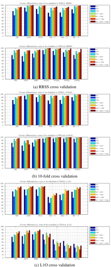
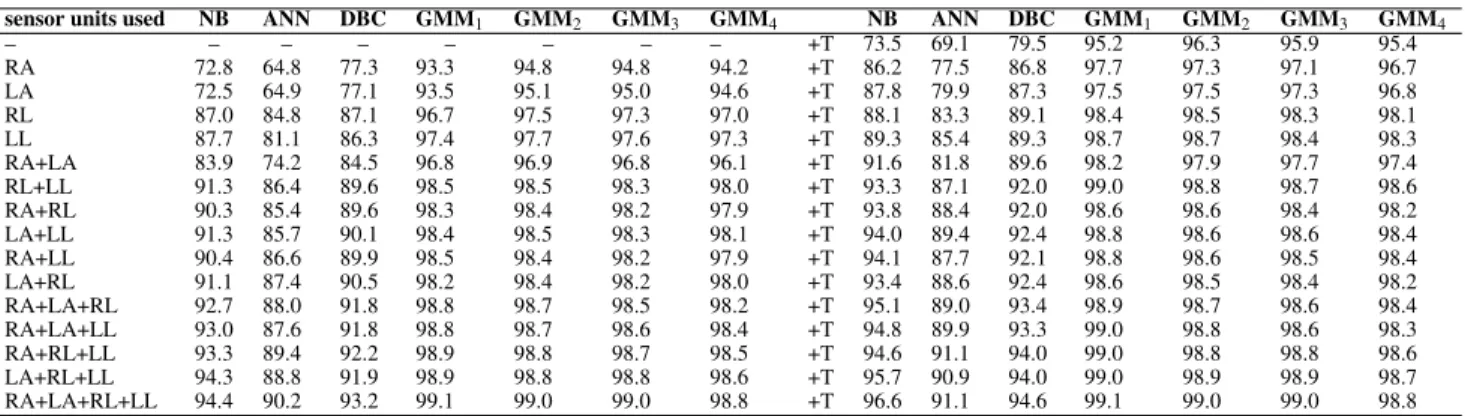
The classification techniques are tested based on every combi-nation of the different sensor types [accelerometer (acc), gyroscope (gyro), and magnetometer (mag)] and sensor units [worn on right arm (RA), left arm (LA), torso (T), right leg (RL), and left leg (LL)]. In the first approach, training data extracted from all possible com-binations of sensor types are used for classification and the results are presented in two different forms. Figure 1 depicts the correct differentiation rates in the form of a bar chart for all possible com-binations of different sensor types using the three cross-validation techniques. Table 1 shows the correct differentiation rates and the standard deviations of the classifications made using the feature vectors extracted from the combination of all sensors. In the sec-ond approach, the training data extracted from all possible combi-nations of different sensor units are used for the tests and correct differentiation rates for only 10-fold cross validation are tabulated in Tables 2 and 3.

classification cross validation

techniques RRSS 10-fold L1O

WEKA NB 93.9±0.49 93.7±0.08 89.2± 5.60 ANN 99.0±0.09 99.0±0.08 90.3± 5.97 SVM 98.1±0.11 98.9±0.03 90.7± 4.83 tree methods NB-T 94.6±0.68 94.9±0.16 67.7± 6.35 J48-T 93.8±0.73 94.5±0.17 77.0± 7.06 RF-T 98.3±0.24 98.6±0.05 86.8± 5.71 PRTools NB 96.5±0.46 96.6±0.07 83.8± 0.63 ANN 92.6±3.10 91.1±3.02 84.7± 3.85 DBC 94.7±0.60 94.6±0.33 89.0± 4.50 GMM GMM1 99.1±0.20 99.1±0.02 76.4± 8.71 GMM2 98.8±0.17 99.0±0.04 48.1± 8.47 GMM3 98.2±0.30 99.0±0.06 37.6±10.25 GMM4 97.3±0.37 98.8±0.08 37.0± 9.21

Table 1: Correct differentiation rates and the standard deviations based on feature vectors extracted from all sensors signals.

It is observed that the 10-fold cross validation has the best per-formance, RRSS following it with slightly smaller rates (Table 1). The cause of the difference is that in 10-fold cross validation, a larger data set is used for training. On the other hand, L1O has the smallest rates and largest standard deviation values in all cases because each subject performs the activities in a different manner. Outcomes obtained by implementing L1O illustrate that the train-ing data should be sufficiently comprehensive in terms of the diver-sity of the physical characteristics of the subjects. Each additional subject with distinctive characteristics included in the initial feature vector set will improve the correct classification rate of newly intro-duced feature vectors.

Compared to other decision-tree methods, random forest out-performs in all of the cases since the random forest consists of 10 decision trees each voting individually for a certain class and the class with the highest vote is classified to be the correct one. In spite of its random nature, it competes with the other classifiers and achieves an average correct differentiation rate of 98.6% for 10-fold cross validation when data from all sensors is used (Table 1). NB-T method seems to be the worst of all decision trees. WEKA provides large number of decision-tree methods to choose from. However, some of these such as best-first and logistic model decision-tree classifiers are not applicable in our case because of the size of the training set, especially for 10-fold cross validation.

Generally, the best performance is expected from SVM and

(a) RRSS cross validation

(b) 10-fold cross validation

(c) L1O cross validation

Figure 1: Comparison of classifiers and combinations of different sensor types in terms of correct differentiation rates.

ANN for problems involving multi-dimensional and continuous feature vectors. L1O cross-validation results for the combination of different sensor types indicate that these classifiers are capable of generalization and are less susceptible to overfitting than other classifiers; especially, the GMM. ANN and SVM classifiers usually have slightly lower performance than GMM1(99.1%) with 99.0% and 98.9%, respectively, for 10-fold cross validation when the fea-ture vectors extracted from combination of all sensors are used for

sensor units used NB ANN SVM NB-T J48-T RF-T NB ANN SVM NB-T J48-T RF-T – – – – – – – +T 71.5 94.4 89.1 77.5 78.2 89.4 RA 67.3 93.2 88.5 80.5 79.7 89.8 +T 82.7 96.9 95.0 87.1 86.1 95.2 LA 70.0 92.8 88.0 76.0 76.6 88.5 +T 83.5 96.9 94.8 87.8 86.3 95.7 RL 87.5 97.3 94.3 86.1 86.3 93.2 +T 86.4 98.1 95.6 90.0 89.4 96.4 LL 87.0 97.7 94.3 87.1 87.7 93.2 +T 86.1 98.3 96.7 89.9 89.9 96.6 RA+LA 79.1 95.3 93.0 87.4 86.3 94.9 +T 87.9 98.0 96.3 91.4 90.0 97.0 RL+LL 89.0 98.2 96.0 91.2 92.1 96.6 +T 91.0 98.6 97.2 93.3 93.1 97.7 RA+RL 89.2 98.0 95.8 90.4 90.6 96.7 +T 90.5 98.3 97.3 92.7 91.4 97.6 LA+LL 90.2 98.2 96.8 90.1 90.1 96.5 +T 92.2 98.5 97.5 92.0 92.0 97.7 RA+LL 89.2 98.3 96.2 90.3 90.1 96.7 +T 90.8 98.5 97.4 92.7 91.8 97.6 LA+RL 90.6 97.7 96.6 90.3 89.5 96.4 +T 91.2 98.4 97.6 92.5 91.4 97.7 RA+LA+RL 91.1 98.7 97.1 92.2 92.0 97.8 +T 93.2 98.9 97.9 94.1 92.8 98.1 RA+LA+LL 90.9 98.7 97.1 92.8 92.3 97.8 +T 92.4 98.9 97.9 93.2 93.1 98.1 RA+RL+LL 91.2 98.7 97.2 93.7 93.0 97.9 +T 93.0 98.8 98.0 94.6 94.3 98.4 LA+RL+LL 91.5 98.6 97.3 94.0 93.7 98.0 +T 93.0 98.8 98.0 94.6 94.3 98.4 RA+LA+RL+LL 92.4 98.8 97.8 95.0 94.3 98.6 +T 93.7 99.0 98.9 94.9 94.5 98.6 Table 2: All possible combinations of different sensor units and the corresponding correct classification rates for classification methods in WEKA using 10-fold cross validation.

sensor units used NB ANN DBC GMM1 GMM2 GMM3 GMM4 NB ANN DBC GMM1 GMM2 GMM3 GMM4

– – – – – – – – +T 73.5 69.1 79.5 95.2 96.3 95.9 95.4 RA 72.8 64.8 77.3 93.3 94.8 94.8 94.2 +T 86.2 77.5 86.8 97.7 97.3 97.1 96.7 LA 72.5 64.9 77.1 93.5 95.1 95.0 94.6 +T 87.8 79.9 87.3 97.5 97.5 97.3 96.8 RL 87.0 84.8 87.1 96.7 97.5 97.3 97.0 +T 88.1 83.3 89.1 98.4 98.5 98.3 98.1 LL 87.7 81.1 86.3 97.4 97.7 97.6 97.3 +T 89.3 85.4 89.3 98.7 98.7 98.4 98.3 RA+LA 83.9 74.2 84.5 96.8 96.9 96.8 96.1 +T 91.6 81.8 89.6 98.2 97.9 97.7 97.4 RL+LL 91.3 86.4 89.6 98.5 98.5 98.3 98.0 +T 93.3 87.1 92.0 99.0 98.8 98.7 98.6 RA+RL 90.3 85.4 89.6 98.3 98.4 98.2 97.9 +T 93.8 88.4 92.0 98.6 98.6 98.4 98.2 LA+LL 91.3 85.7 90.1 98.4 98.5 98.3 98.1 +T 94.0 89.4 92.4 98.8 98.6 98.6 98.4 RA+LL 90.4 86.6 89.9 98.5 98.4 98.2 97.9 +T 94.1 87.7 92.1 98.8 98.6 98.5 98.4 LA+RL 91.1 87.4 90.5 98.2 98.4 98.2 98.0 +T 93.4 88.6 92.4 98.6 98.5 98.4 98.2 RA+LA+RL 92.7 88.0 91.8 98.8 98.7 98.5 98.2 +T 95.1 89.0 93.4 98.9 98.7 98.6 98.4 RA+LA+LL 93.0 87.6 91.8 98.8 98.7 98.6 98.4 +T 94.8 89.9 93.3 99.0 98.8 98.6 98.3 RA+RL+LL 93.3 89.4 92.2 98.9 98.8 98.7 98.5 +T 94.6 91.1 94.0 99.0 98.8 98.8 98.6 LA+RL+LL 94.3 88.8 91.9 98.9 98.8 98.8 98.6 +T 95.7 90.9 94.0 99.0 98.9 98.9 98.7 RA+LA+RL+LL 94.4 90.2 93.2 99.1 99.0 99.0 98.8 +T 96.6 91.1 94.6 99.1 99.0 99.0 98.8

Table 3: All possible combinations of different sensor units and the corresponding correct classification rates for classification methods in PRTools using 10-fold cross validation.

classification (Table 1). In the case of L1O cross validation, their success rates are significantly better than GMM1.

Considering the outcomes obtained using 10-fold cross valida-tion and based on the combinavalida-tions of different sensor types, it is difficult to determine the number of mixture components to be used in the GMM classifier. The average correct differentiation rates are quite close to each other for the GMM1, GMM2, and GMM3 (Gaus-sian mixture models with 1, 2, and 3 components). However, in the case of RRSS and especially L1O cross validation, the rates rapidly decrease as the number of components in the mixture increases. The reason for such an outcome would be overfitting. While multiple Gaussian estimators are exceptionally complex for classification of training patterns, they are unlikely to give accurate classification of novel patterns. The low differentiation rates of GMM classifier for L1O cross validation supports this interpretation. Despite the in-competent outcomes taken from GMM classifier for L1O case, it is the best classifier with 99.1% average correct differentiation rate based on 10-fold cross validation (Table 1).

The comparison of classification results based on the combina-tions of different sensor types reveals that when the data set corre-sponding to magnetometers alone is used, the average correct differ-entiation rate is higher than the rates obtained by the other two sen-sor types used alone (Figure 1). Furthermore, in most of the cases, the rate provided by magnetometer data alone outperforms the rates provided by two sensors combined together. Indeed, in Figure 1, for almost all classification methods evaluated based on all cross-validation techniques, the turquoise bar is higher than the green bar except for the GMM model tested with L1O cross validation. The best performance (98.3%) based on the magnetometer data is achieved with ANN using 10-fold cross validation (Figure 1(b)).

Correct differentiation rates obtained by using feature vectors based on the gyroscope data are the lowest (Figure 1). Outcomes of the combination of gyroscope with other two sensors are also worse than the combination of accelerometer and magnetometer. The magnetometers used in this study function as a magnetic com-pass. Thus, the results indicate that the most informative features are extracted from the compass data (magnetometer), followed by the translational data (accelerometer), and, finally, the rotational data (gyroscope).

The case in which classifiers are tested based on the combi-nations of different sensor units shows that the GMM method has the best classification performance for all combinations and cross-validation techniques other than L1O (Tables 2 and 3). In L1O cross validation, SVM has the best performance. When a single unit or a combination of two units is used in the tests, correct differentiation rates achieved with GMM2are better than GMM1. Furthermore, the sensor units placed on the legs (RL and LL) seem to provide the most useful information. Comparing the cases where the feature vectors extracted from a single sensor unit data, it is observed that the highest correct classification rates are achieved with these two units. They also improve the performance of the combinations in which they are included.

The performances of the classifiers implemented are compared in terms of their execution times. The master software MATLAB is run on a computer with Pentium(R) Dual-Core CPU E520 at clock frequency of 2.50 GHz, 2.00 GB of RAM, and operated with Mi-crosoft Windows XP Home Edition. Execution times for training and test steps corresponding to all classifiers and both environments are provided in Table 4. These are based on the time it takes for full L1O cross-validation cycle to be completed. In other words, each

classification time (sec)

techniques training test

WEKA NB 1.66 20.44 ANN 2416.00 4.50 SVM 69.04 5.68 tree methods NB-T 2610.90 2.65 J48-T 24.09 2.65 RF-T 57.47 2.80 PRTools NB 0.68 0.48 ANN 547.77 0.44 DBC 98.55 1.41 GMM GMM1 1.33 0.46 GMM2 161.70 0.58 GMM3 129.44 0.72 GMM4 118.02 1.06

Table 4: Execution times of training and test steps based on the full cycle of L1O cross-validation technique.

classifier is run 8 times for all subjects and the total time of the complete cycle for each classifier is recorded. Assuming that these classification algorithms are used in a real-time system, it is desir-able to keep the test times at a minimum.

In comparing the two machine learning environments used in this study, algorithms implemented in WEKA appear to be more robust to parameter changes than PRTools. In addition, WEKA is easier to work with because of its graphical user interface (GUI). The interface displays detailed descriptions of the algorithms along with their references and parameters when needed. On the other hand, PRTools does not have a GUI and the descriptions of the al-gorithms given in the references are insufficient.

The implementations of the same algorithm in WEKA and PRTools may not be exactly the same. For instance, this is reflected by the difference in correct differentiation rates obtained with NB and ANN classifiers. The higher rates are achieved with NB imple-mented in PRTools because the distribution of each feature is esti-mated with histograms. On the other hand, WEKA uses a normal distribution to estimate probability density functions. Considering the ANN classifier, PRTools does not allow the user to set values for the learning and momentum constants which play a crucial role in updating the connection weights. Therefore, the ANN implemented in PRTools is quite incompetent compared to the one implemented in WEKA.

In terms of the correct differentiation rates, training, and test times, GMM1 is superior to the other methods with a few excep-tions. An alternative to GMM technique would be SVM and ANN techniques. Among the decision-tree methods, because it trains a NB classifier for every leaf node, NB-T has the longest training time, whereas J48-T has the shortest. There is hardly a difference between the test times of decision-tree methods. Therefore, taking its high correct classification rate into consideration, RF-T seems to be the best decision-tree learner. The DBC with its moderate correct classification rates and relatively long test time is not to be preferred among PRTools classifiers.

The results previously published by our group (using our own codes) indicate that the best method, with its high correct classi-fication rate and relatively small pre-processing and classiclassi-fication times is Bayesian decision making (BDM) [10]. In 10-fold cross-validation scheme, it has a rate of 99.2% which outperforms ev-ery classifier used in this study with a slight difference (0.1% for GMM1). On the other hand, rates obtained by using ANN and SVM presented in this study are up to 3% higher than the ones provided in [10]. These differences arise both from the implementation of the algorithms and the variation in the distribution of the feature vectors in the partitions obtained by cross-validation techniques. The high rates provided by BDM and GMM1in these studies illustrate the high classification accuracy of multi-variate Gaussian models for activity recognition tasks.

4. CONCLUSION

We presented the results of a comparative study in which features extracted from miniature inertial sensor and magnetometer signals are used for classifying human activities. Several classification techniques are compared based on the same data set in terms of their correct classification rates and computational costs.

In general, the correct classification rate achieved by the GMM1 technique is higher and this technique requires quite small computa-tional time compared to other classification techniques. The GMM technique seems to be a suitable method for activity classification problems. The ANN and SVM are the second-best choices in terms of classification performance; however, the computational cost of these methods is very high.

The magnetometer turns out to be the best type of sensor to be used in classification where gyroscope is the least useful compared to the other sensor types. However, it should be kept in mind that the absolute information that magnetometer signals provide can be distorted by metal surfaces and magnetized objects in the vicinity of the sensor. Considering the positioning of the sensor units on body, the sensors worn on the legs seem to provide the most valuable in-formation on activities.

5. ACKNOWLEDGEMENT

This work is supported by the Scientific and Technological Re-search Council of Turkey under grant number EEEAG-109E059.

REFERENCES

[1] S. J. Preece, J. Y. Goulermas, L. P. J. Kenney, D. Howard, K. Meijer, and R. Crompton, “Activity identification using body-mounted sensors—a review of classification techniques,” Physiol. Meas., 30(4):R1–R33, Apr. 2009.

[2] J. P¨arkk¨a, M. Ermes, P. Korpip¨a¨a, J. M¨antyj¨arvi, J. Peltola, and I. Korhonen, “Activity classification using realistic data from wearable sensors,” IEEE Trans. Inform. Technol. Biomed., 10(1):119–128, Jan. 2006.

[3] K. Aminian, P. Robert, E. E. Buchser, B. Rutschmann, D. Hayoz, and M. Depairon, “Physical activity monitoring based on accelerometry: validation and comparison with video observation,” Med. Biol. Eng. Comput., 37(1):304–308, Dec. 1999.

[4] L. Bao and S. S. Intille, “Activity recognition from user-annotated acceleration data,” in Proc. Pervasive Computing, Lect. Notes Comput. Sci., Vienna, Austria, 21–23 April 2004, pp. 1–17.

[5] M. J. Mathie, B. G. Celler, N. H. Lovell, and A. C. F. Coster, “Classification of basic daily movements using a triaxial ac-celerometer,” Med. Biol. Eng. Comput., 42(5):679–687, Sept. 2004.

[6] N. Kern, B. Schiele, and A. Schmidt, “Multi-sensor activity context detection for wearable computing,” in Proc. EUSAI 2003, Eindhoven, The Netherlands, 3–4 Nov. 2003, pp. 220– 232.

[7] R. O. Duda, P. E. Hart, and D. G. Stork, Pattern Classification, New York: John Wiley & Sons, Inc., 2001.

[8] M. Hall, E. Frank, G. Holmes, B. Pfahringer, P. Reutemann, and I. H. Witten, “The WEKA data mining software: an up-date,” ACM SIGKDD Explorations Newsletter, 11(1):10–18, June 2009.

[9] R. P. W. Duin, P. Juszczak, P. Paclik, E. Pekalska, D. de Rid-der, D. M. J. Tax, S. Verzakov, PRTools 4.1 A Matlab Toolbox for Pattern Recogn., Delft University of Technology, Delft, The Netherlands, Aug. 2007.

[10] K. Altun, B. Barshan, and O. Tunel, “Comparative study on classifiying human activities with miniature inertial and mag-netic sensors,” Pattern Recogn., 43(10):3605–3620, April 2010.