A privacy-preserving solution for the bipartite ranking problem on spark framework

A PRIVACY-PRESERVING SOLUTION FOR

THE BIPARTITE RANKING PROBLEM ON

SPARK FRAMEWORK

a thesis submitted to

the graduate school of engineering and science

of bilkent university

in partial fulfillment of the requirements for

the degree of

master of science

in

computer engineering

By

Noushin Salek Faramarzi

July 2017

A Privacy-Preserving Solution for the Bipartite Ranking Problem on Spark Framework

By Noushin Salek Faramarzi July 2017

We certify that we have read this thesis and that in our opinion it is fully adequate, in scope and in quality, as a thesis for the degree of Master of Science.

Altay Güvenir(Advisor)

Erman Ayday

Engin Demir

Approved for the Graduate School of Engineering and Science:

Ezhan Karaşan

ABSTRACT

A PRIVACY-PRESERVING SOLUTION FOR THE

BIPARTITE RANKING PROBLEM ON SPARK

FRAMEWORK

Noushin Salek Faramarzi M.S. in Computer Engineering

Advisor: Altay Güvenir July 2017

The bipartite ranking problem is defined as finding a function that ranks positive

instances in a dataset higher than the negative ones. Financial and medical

domains are some of the common application areas of the ranking algorithms. However, a common concern for such domains is the privacy of individuals or companies in the dataset. That is, a researcher who wants to discover knowledge from a dataset extracted from such a domain, needs to access the records of all individuals in the dataset in order to run a ranking algorithm. This privacy concern puts limitations on the use of sensitive personal data for such analysis. We propose an efficient solution for the privacy-preserving bipartite ranking problem, where the researcher does not need the raw data of the instances in order to learn a ranking model from the data.

The RIMARC (Ranking Instances by Maximizing Area under the ROC Curve) algorithm solves the bipartite ranking problem by learning a model to rank in-stances. As part of the model, it learns a weight for each feature by analyzing the area under receiver operating characteristic (ROC) curve. RIMARC algorithm is shown to be more accurate and efficient than its counterparts. Thus, we use this algorithm as a building-block and provide a privacy-preserving version of the RIMARC algorithm using homomorphic encryption and secure multi-party computation.

In order to increase the time efficiency for big datasets, we have implemented privacy-preserving RIMARC algorithm on Apache Spark, which is a popular par-allelization framework with its revolutionary programming paradigm called Re-silient Distributed Datasets.

iv

Our proposed algorithm lets a data owner outsource the storage and processing of its encrypted dataset to a semi-trusted cloud. Then, a researcher can get the results of his/her queries (to learn the ranking function) on the dataset by interacting with the cloud. During this process, neither the researcher nor the cloud can access any information about the raw dataset. We prove the security of the proposed algorithm and show its efficiency via experiments on real data.

ÖZET

İKİ TARAFLI SIRALAMA PROBLEMİNE SPARK

ÇERÇEVESİNDE GİZLİLİĞI KORUYAN BİR ÇÖZÜM

Noushin Salek Faramarzi

Bilgisayar Mühendisliği, Yüksek Lisans Tez Danışmanı: Halil Altay Güvenir

Temmuz 2017

İki uçlu sıralama problemi, bir veri kümesindeki pozitif örnekleri negatif olan-lardan daha yüksek konumlara yerleştiren bir fonksiyon bulma problemi olarak tanımlanır. Finansal ve tıbbi alanlar, sıralama algoritmalarının ortak uygulama alanlarından bazılarıdır. Bununla birlikte, bu tür alanlar için ortak bir endişe, veri kümesindeki kişilerin mahremiyetidir. Yani, böyle bir alandan elde edilen bir veri kümesindeki bilgiyi keşfetmek isteyen bir araştırmacı bir sıralama algoritması çalıştırmak için veri kümesindeki bireylerin tüm bilgilerine erişmek zorundadır. Gizlilik endişesi, bu tür analizler için hassas kişisel verilerin kullanımına ilişkin sınırlamalar getirmektedir. Araştırmacının, verilerden bir sıralama modeli öğren-mek için örneklerin ham verilerine ihtiyaç duymadığı, gizliliği koruyan iki uçlu sıralama problemi için verimli bir çözüm önermekteyiz.

RIMARC (ROC Eğrisi Altındaki Alanı Maksimize Ederek Örnekleri Sıralama) algoritması, örnekleri sıralamak için bir model öğrenerek iki uçlu sıralama prob-lemini çözer. Modelin bir parçası olarak, alıcının çalışma karakteristiği (ROC) eğrisi altındaki alanı analiz ederek her bir özellik için bir ağırlık öğrenir. RI-MARC algoritmasının benzer sıralama algoritmalarından daha başarılı ve hızlı olduğu gösterilmiştir. Dolayısıyla, RIMARC algoritmasını bir yapı taşı olarak alıp, homomorfik şifreleme ve güvenli çok partili hesaplama kullanarak bu algo-ritmanın gizliliği koruyan bir versiyonunu geliştirdik.

RIMARC algoritmasının büyük veri kümelerinde zaman verimliliğini artırmak için, Resilient Distributed Datasets adlı programlama paradigması ile popüler, bir paralelleştirme çerçevesi olan Apache Spark’da gizliliği koruyan versiyonunu geliştirdik.

vi

ve işlenmesini, yarı güvenilir bir bulut ortamında dış kaynak olarak sağlar. Bir araştırmacı, bir sıralama fonksiyonu öğrenmek için bulut ile etkileşim kurarak veri kümesindeki sorgularının sonuçlarını alabilir. Bu süreçte ne araştırmacı ne de bulut, işlenmemiş veri kümesiyle ilgili herhangi bir bilgiye erişemez. Önerilen algoritmanın güvenliği kanıtlanmakta ve gerçek veriler üzerindeki deneyler ile verimliliği gösterilmektedir.

Anahtar sözcükler : İki Taraflı Sıralama Problemi, Veri Madenciliği, Veri gizliliği, Spark.

Acknowledgement

I would like to express my sincere gratitude to my advisor Prof. Dr. Altay Güvenir for his support, suggestions, encouragement and guiding me through this study. It was a great pleasure for me to work with him in this thesis and I want to express my great respect to him for giving me a chance to work with him.

And I would like to thank Prof. Dr. Erman Ayday for supporting and men-toring me. I am thankful for his guidance and motivation in each and every way. Also, I would like to thank Prof. Dr. Engin Demir for accepting to read and review this thesis.

Also I would like to thank my friends; Caner for being nice and humble, Ali Burak, Başak, Iman, Istemi, Mohammad, Nazanin, Onur, Saharnaz, Simge and Troya for all of the great memories. I will never forget the enjoyable time we have had together. I would like to thank dear Hamed and dear Negin for their valuable emotional support and helping in the time that I need them. Nothing would be the same without you.

I can not forget the kindness of our department sweet heart Ebru Ateş. A great thanks for being nice and helpful.

I would like to thank my parents, my sister (Naim), my brother (Naser) and my little princess (Nardin) for their love and support that always kept me motivated. None of my achievements would have been possible without your support.

Contents

1 Introduction 1

2 Background 6

2.1 Receiver Operating Characteristic Curve . . . 6

2.2 Area Under the ROC Curve . . . 9

2.2.1 Properties of ROC and AUC . . . 9

2.3 RIMARC Algorithm . . . 12

2.4 Homomorphic Encryption . . . 15

2.4.1 Encryption . . . 16

2.4.2 Decryption . . . 17

2.4.3 Properties Of The Paillier Cryptosystem . . . 17

2.5 Open Source Software for Processing of Big Data . . . 20

2.5.1 MapReduce . . . 20

CONTENTS ix

2.6 Spark . . . 27

2.6.1 Resilient Distributed Dataset . . . 27

3 Proposed Solution 30 3.1 System and Threat Models . . . 30

3.2 Dataset Format and Encryption . . . 32

3.3 Privacy-Preserving RIMARC Algorithm . . . 33

3.4 Security Evaluation . . . 37

3.5 Evaluation . . . 38

4 Spark Implementation 41 4.1 Experiment Setup . . . 45

4.2 Evaluation . . . 45

List of Figures

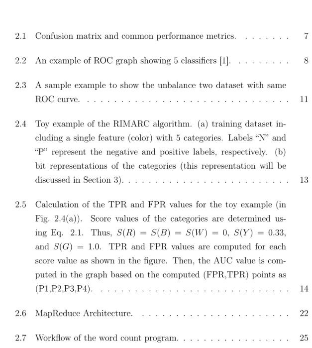
2.1 Confusion matrix and common performance metrics. . . 7

2.2 An example of ROC graph showing 5 classifiers [1]. . . 8

2.3 A sample example to show the unbalance two dataset with same

ROC curve. . . 11

2.4 Toy example of the RIMARC algorithm. (a) training dataset

in-cluding a single feature (color) with 5 categories. Labels “N” and “P” represent the negative and positive labels, respectively. (b) bit representations of the categories (this representation will be

discussed in Section 3). . . 13

2.5 Calculation of the TPR and FPR values for the toy example (in

Fig. 2.4(a)). Score values of the categories are determined

us-ing Eq. 2.1. Thus, S(R) = S(B) = S(W ) = 0, S(Y ) = 0.33, and S(G) = 1.0. TPR and FPR values are computed for each score value as shown in the figure. Then, the AUC value is com-puted in the graph based on the comcom-puted (FPR,TPR) points as

(P1,P2,P3,P4). . . 14

2.6 MapReduce Architecture. . . 22

LIST OF FIGURES xi

2.8 Workflow of the word count program using Spark. . . 29

3.1 Proposed system model. . . 31

3.2 Overview of the proposed solution. Steps 3, 5, and 6 are interactive

steps between the cloud and the researcher. . . 34

4.1 Run time of the privacy-preserving RIMARC algorithm using

List of Tables

3.1 Time complexity of the proposed algorithm for different sizes of the

security parameter (n), different number of features in the dataset,

and different database sizes. . . 39

4.1 A toy example of calculating total number of each category. . . . 42

4.2 Adding noise to the bits and labels in order to send to researcher. 43

Chapter 1

Introduction

Data mining has become an emerging and rapidly growing field in recent years because of the increases in the ability to store data and explosive development in networking. Analysis of data is performed after collecting and storing data. These progresses led to creation of large amount of data which are stored in unprecedented way in databases. However, the helpfulness of this information is questionable if "meaningful information" can not be extracted out of it [2]. Data mining is a way for looking large amount of data to discover meaningful patterns and trend out of raw data. The data mining brings insights into mess data and investigates explicit information to assist decision-making for many organizations. Being aware of specific patterns in domains such as finance or medicine play an important role in saving money and lives, respectively. However, traditional data mining algorithms operated on original dataset, which led to emergence of concerns about data privacy. In the meantime, huge amount of data involves the sensitive knowledge that their exposure can not be overlooked to the competitiveness of enterprise.

In addition, World Wide Web provides a platform that collecting data and adding them to the databases become easy. As a result of that, privacy issues are further exacerbated. Considering recent changes, the beneficial research on data mining will be the development of techniques that incorporate privacy.

The main objective of the privacy-preserving data mining is to decrease the risk of misuse of original data and produce the same high quality results the way that it would be in the absence of privacy-preserving technique [3, 4].

In another word, Privacy-Preserving Data Mining (PPDM) is to provide ex-pected level of privacy preservation to the data mining related computations and processes. PPDM is designed to protect personal and sensitive data from di-vulging to the general population without the providers’ consent in the process of data mining [5]. It is needed to have privacy protection in real life.

Data providers are not interested in sharing the data because of the problem of privacy disclosure. In another side, business holders concern about the sensi-tivity of their secret financial information. For an instance, telecommunication customers are not interested in sharing their phone call list and business partners are also do not want to share these important information in the process of data mining. On top of that, privacy protection of the medical data is taken more seriously than other data mining because medical records are related to human subjects.

Ethical health research and privacy protections both provide valuable benefits to society. Health research is vital to improving human health and health care. It is essential to protect patients from harm and preserve their rights in ethical research. Therefore, PPDM is a very important issue that should be solved in the applications related to data analysis, especially in medical domain [6, 7].

In order to achieve privacy-preserving data mining several techniques can be utilized such as Trust Third Party, Data perturbation, game theoretic approach, Secure Multiparty Computation and Data perturbation. But, for an instance in Multiparty Computation technique, there is a thought that the environment that we have is semi-honest. As a result of that, the parties will always follow the protocol and never attempt to collide [6].

Participants in distributed data mining is assumed to be semi-honest, but we should not ignore the fact that there may be additional advantages in collision of

parties. So there has to be inclination privacy-preserving data mining to construct protocol or algorithms that will be collusion resistant.

The topics of the Secret Sharing technique, the Homomorphic Threshold Cryp-tography and the protocols based on the penalty function mechanism have dis-cussed in [8–10] that can address the aforementioned issues.

This thesis focuses on bipartite ranking problems and proposes an algorithm

that efficiently solves the problem in a privacy-preserving manner. Bipartite

ranking have received considerable attention from machine learning community recently. In these problems, we try to find a score function that assigns a value to each instance, such that positive instances have a higher score than the negative ones. In order to do that we use a training set where the instances have positive and negative labels. When the resulting ranking function is applied to a new unlabeled instance, the function is expected to establish a total order in which positive instances precede negative ones [11]. The most commonly used criterion for measuring the performance of a score function in bipartite ranking is the area under the receiver operating characteristic (ROC) curve (known as AUC) that will be discussed in Section 2.2.

Several application can be considered for bipartite ranking. For example, in content recommendation we are trying to have a ranking function that rank the set of items based on the individual’s interests or another example can be epi-demiological studies in which we are trying to rank the individuals based on their likelihood to have a specific disease [12].

One common drawback of the algorithms that solve the bipartite ranking prob-lem is their applicability in real-life settings. This drawback arises due to privacy sensitivity of personal data that is collected by the data owner. This is an issue for all machine learning research where a real life dataset is used for training. As mentioned earlier, protecting patient’s privacy from an untrusted third party and preserving their rights is necessary for ethical research. In contrast, the primary justification for collecting personally identifiable health information for health

research is to benefit society. Because it allows complex activities, including re-search and public health activities to be done in ways that protect individuals’ dignity. In the meantime, health research can benefit individuals, for example, new improvements in diagnostics and access to new therapies will help patients to prevent illness.

In most cases, the data owner (that collects and labels the data) does not have sufficient resources (i.e., storage and computation power) to answer the queries (to learn a ranking function on the dataset) of the researchers about the dataset. For instance, most researchers request sensitive medical information from hospitals to work on, but privacy concerns make the hospitals unwilling to provide such information.

On the one hand, getting the result of such queries and learning the ranking function is very valuable for the researchers in most cases. On the other hand, the data owner does not directly share its own dataset with the researcher due to the aforementioned privacy and legal concerns. Therefore, usually, the data owner has two options:

(i) the data owner may anonymize the dataset before sharing it with the re-searchers, which reduces the utility and accuracy of the dataset, and hence the query result.

(ii) it can outsource the storage and processing of the dataset to a trusted party, however existence of such a trusted party is not practical in most real-life settings.

In this thesis, we focus on the latter option, but rather than assuming the existence of a fully trusted party, we resort to using cryptographic techniques. We use the RIMARC algorithm as a building-block and propose a privacy-preserving version of the RIMARC algorithm [11]. To achieve our goal, we use Homomorphic encryption [13] and secure multi-party computation.

Furthermore, the parallelizable feature of the RIMARC algorithm lead us to investigate this aspect of algorithm to evaluate the performance of the algorithm

while protecting the privacy of RIMARC algorithm. In order to accomplish this, we used clustering computing framework called Spark, which have the same prop-erties of fault tolerance and scalability of MapReduce [14].

One of the key concept in Spark is using Resilient Distributed datasets (RDDs) [15]. RDDs are in-memory data structures that cache intermediate data across the several nodes. The main reason that makes time very efficient is the locality of the RDDs in memory. So, it provides an ability to iterate over RDD as many times as needed.

The proposed algorithm ensures that no party other than the data owner can access to the content of the dataset. Furthermore, the researchers can only obtain the results of their queries, and the cloud can not learn anything about the dataset. We prove the security of the proposed algorithm and show its efficiency via experiments on real data.

The rest of the Thesis is organized as follows. In the next section, we provide background information about the RIMARC algorithm and the cryptographic tools we use in our algorithm. In Section 3, we describe our proposed privacy-preserving algorithm in detail and we also provide a brief security analysis. In Section 4, we discuss the Spark implementation. Finally, in Section 5, we conclude the paper and discuss potential future works.

Chapter 2

Background

In this chapter, the background information for learning the concept is provided. The ROC and AUC subjects are given since they are essential in RIMARC and Homomorphic encryption and Spark framework are discussed as well.

2.1

Receiver Operating Characteristic Curve

Receiver Operating Characteristic (ROC) curve is a well-known tool for evalu-ating the performance of binary classifiers. It is a powerful metric compared to traditional accuracy metrics. The first application of ROC graphs dates back to World War II, the research was about make sense out of noisy signals [16]. The first application to machine learning is done by Spackman [17]. According to Fawcett’s definition, the ROC graph is a tool that can be used to visualize, organize and select classifiers based on their performance [1].

This metric is mainly used in medical decision making, and nowadays there is a gradual increase in the usage of this metric in machine learning and data mining communities. It has become a popular performance measure in these communities because it has been realized that accuracy is not a sufficient metric to evaluate the performance of a classifier [1, 18–20].

ROC curve is usually used in binary classifiers, two classifier with two possible output classes. Some classifiers estimate the probability of an instance’s label and some other classifiers map from instances to predicted classes. Output of a discrete classifier is represented by only one point on ROC space, because one confusion matrix is generated from their classification output. Some classification models produce continuous output by estimating the instance’s class membership probability. In these models, instead of one confusion matrix we have many confusion matrices which are produced by applying various thresholds in order to predict class membership. Therefore, distinct confusion matrices are obtained as a result of these threshold values. As a result, number of confusion matrix is equal to number of ROC points on a ROC space.

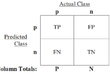
There are four types of outputs in binary prediction. A true positive rate output is one that correctly predicts the class while the class label is positive. A False Positives rate output is one that incorrectly predicts the class while the class label is positive. A True Negative rate output is one that correctly predicts the class while the class label is negative. A False Negative rate output is one that incorrectly predicts the class while the class label is negative.

Figure 2.1: Confusion matrix and common performance metrics.

graphs the most important elements are TP and FP which are used to calculate FPR and TPR where N is the number of total negative instances and P is number of total positive instances.

As it can be seen in Fig. 2.2, ROC graphs are two-dimensional graphs which are generated by plotting TPR on Y axis and FPR on X axis at different threshold values. As mentioned above, each discrete classifier produces a (FPR,TPR) pair, which corresponds to a single point in the ROC space. A perfect classifier yields a point on the upper left corner coordinate (0, 1) of the ROC space. On the other hand, a completely random guess would give a point along a diagonal line from the left bottom to the top right corners towards (0.5, 0.5).

Figure 2.2: An example of ROC graph showing 5 classifiers [1].

The best classifier among the ones in Fig. 2.2 is D classifier. The points that are located on upper left of the space perform better than the other points because of the fact that TP rate is higher and/or FP rate is lower. The classifiers that are located on left-hand side of the ROC graph, near the horizontal axis they often make fewer false positive errors and low true positive rates as well. The

classifiers that are appearing on the right-hand side of an ROC graph guess most of the positives instances correctly, but they often have high false positive rates. Considering the fact that most of the real life problem have negative instances more often, it is logical to work on far left-hand side of the graph.

2.2

Area Under the ROC Curve

As mentioned, the ROC graph is used to visualize the performance of a classifier, some classifier use a threshold for predicting the class label of a query instance. Such classifiers compute a value for a query instance first. If this value is greater than the threshold, they predict the label of the instance as positive. If the value is below the threshold the predicted label would be negative. We can use Area Under ROC curve (AUC) measurement to investigate a classifier’s performance that has such a threshold value.

The area under the ROC curve (AUC) is a measure of the probability that a classifier will rank a randomly chosen positive instance higher than a randomly chosen negative instance. The highest possible AUC value is 1.0 which represents a perfect classification, and a value of 0.5 corresponds to a random decision [1]. Therefore, the values below 0.5 can be easily neglected. A feature with a higher AUC value can determine the class label with a higher relevance. AUC is an indicator for quality of ranking and the higher AUC implies better ranking. The main reason why AUC selected as a evaluation metric is because AUC can mea-sure the quality of ranking, it is better than accuracy metric when we consider this factor.

2.2.1

Properties of ROC and AUC

In real world, most of the problems do not have balanced classes. However, unbal-anced data does not affect how ROC curve is generated. Furthermore, predicted probabilities are unlikely to have a "smooth" distribution. It is important to note

that, ROC curve and AUC can remain indifferent to the calibration of predicted probabilities and actually represented probabilities of class membership.

In other words, As far as we keep the same ordering of observations by pre-dicted probability, ROC curve and AUC will be equal for the cases with different predicted probabilities. For an instance, ROC curve and AUC will be same for predicted probabilities ranged from (0.9 to 1) and (0 to 1). The most important concern of AUC metric is quality of classifier in separating two classes. There-fore, the rank ordering become important. In other words, AUC is a metric that ranks randomly chosen positive instances higher than the randomly chosen neg-ative instances [1]. As a result of that, in highly unbalanced classes, AUC can be used as a useful metric. Broadly, ROC curves are useful even if our predicted probabilities are not "properly calibrated".

Let’s have an example to understand the concept. We have two sample datasets with unbalanced values. At the end we will observe that both of them will have the same AUC value. The AUC value for both of the datasets will be 0.796 and Fig. 2.3 represents the ROC curve of these datasets which indicates that datasets with unbalanced classes can be measured in a well manner using ROC curve.

A B 2 1 5 15 25 2 4 4 ₄₀ N P P N P N P P N P

Figure 2.3: A sample example to show the unbalance two dataset with same ROC curve.

The second point is that, despite the fact that ROC curves are mainly used in binary classification, there are some cases that ROC curves can be extended to the multi class classification. For example if we have three classes, we will have the first class as a positive class and the other two classes group as negative class. Then we change the class labels and select second class as positive and the others and negative then do the same procedure for the third class. Briefly, ROC curves can be extended to problems with three or more classes.

Finally, we need to decide on setting the classification threshold. In this phase, that is more of a business decision. It depends on whether we want to minimize the False Positive Rate or maximize our True Positive Rate. In the end we ourself need to choose a classification threshold, but ROC curve will help us to visually understand the impact of the choice.

2.3

RIMARC Algorithm

Ranking Instances by Maximizing Area under the ROC Curve (RIMARC) learns a ranking function over an instance space. RIMARC algorithm is a binary clas-sification methodology that ranks instances based on how likely to have positive label [11]. In many real life example, we observe that, binary classification can be cast as ranking problem. For example, in movie recommendation system, instead of predicting movie for an individual based on interest, it is more beneficial to provide a ranking list of movies to the user that he/she may enjoy. We can say the same in epidemiological studies in which rather than merely predicting an individual disease probability, it is more helpful to provide a ranking list that represent the likelihood of a patient in having a specific disease [12].

RIMARC is a ranking algorithm that learns a scoring function to maximize the AUC metric. RIMARC finds a ranking function for one categorical feature instead of finding ranking function for whole dataset and then combines theses functions to form one covering all features.

Initially, all continuous features are needed to be discretized to categorical features by MAD2C method [21] in a way that optimizes the AUC. The AUC value, obtained for a single feature shows the effect of that feature in ranking. If the AUC computed for the feature f is 1, that means perfect ordering and this is the maximum value that AUC can have. That is, all instances in the training set can be ranked by using only the values of feature f . Therefore, we expect that query instances can be ranked correctly by using feature f only, as well. An important property of such a ranking function is that it is in a human readable form that can be easily assessed by domain experts. The score value (S) for a

given category j of a specific feature fi, including discretized continuous features,

can be computed as below:

S(cj_i) = P (c

j i)

Here, cj_i represents the jth _{category of feature f}

i. Also, P (cji) and N (c

j

i)

rep-resent the total number of positive and negative instances of cj_i, respectively.

All of the categories (of a given feature) are sorted according to their score val-ues computed in the previous step. Since the ranking function used by RIMARC always results in a convex ROC curve, the AUC is always greater than or equal to 0.5. The ROC curve points, (FPR, TPR), corresponding to each score value is calculated at this step. Using these points, the AUC value is determined. The

weight of a feature, fi is computed as, wi = 2(AU C(i) − 0.5), where AU C(i) is

the AUC obtained for feature fi.

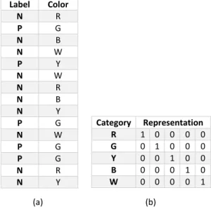
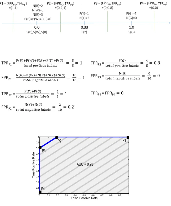
A toy example. To understand how RIMARC works, consider a toy training dataset with a single feature as shown in Fig. 2.4(a). The feature we consider in this example has a total of 5 categories (R, B, W, Y, G). The score values of these categories are obtained, using Eq. 2.1, as follows: S(R) = S(B) = S(W ) = 0, S(Y ) = 0.33, S(G) = 1.0. As shown in Fig. 2.5, the score values are sorted and mapped on an axis. Then, TPR and FPR values calculated for each score value. AUC value is determined using the area under the ROC curve.

Label Color N R P G N B N W P Y N W N R N B N Y P G N W P G P G N R N Y Category Representation R 1 0 0 0 0 G 0 1 0 0 0 Y 0 0 1 0 0 B 0 0 0 1 0 W 0 0 0 0 1 (a) (b)

Figure 2.4: Toy example of the RIMARC algorithm. (a) training dataset includ-ing a sinclud-ingle feature (color) with 5 categories. Labels “N” and “P” represent the negative and positive labels, respectively. (b) bit representations of the categories (this representation will be discussed in Section 3).

0 0.1 0.2 0.3 0.4 0.5 0.6 0.7 0.8 0.9 1 0 0.1 0.2 0.3 0.4 0.5 0.6 0.7 0.8 0.9 1

False Positive Rate

True Positive Rate AUC = 0.98 P1 P2 P3 P4 0 0.1 0.2 0.3 0.4 0.5 0.6 0.7 0.8 0.9 1 0 0.1 0.2 0.3 0.4 0.5 0.6 0.7 0.8 0.9 1

False Positive Rate

True Positive Rate AUC = 0.98 P1 P2 P3 P4

Figure 2.5: Calculation of the TPR and FPR values for the toy example (in Fig. 2.4(a)). Score values of the categories are determined using Eq. 2.1. Thus, S(R) = S(B) = S(W ) = 0, S(Y ) = 0.33, and S(G) = 1.0. TPR and FPR values are computed for each score value as shown in the figure. Then, the AUC value is computed in the graph based on the computed (FPR,TPR) points as (P1,P2,P3,P4).

2.4

Homomorphic Encryption

Encrypted data is required to decrypted sooner or later in order to able to do some analysis. In real life, Keeping cloud files cryptographically scrambled by predefined secret key with the idea that no other third parties will have the required resources to crack them is not applicable. Actually, when there is a need to do some operation like editing text or querying a database of financial data, willingly or not we need to unlock the data. As result of that data become vulnerable. Homomorphic encryption, could change this fact as a pioneer in the science of keeping secrets.

In Homomorphic encryption computation can be done without any require-ment to decrypt the data. Accordingly, complex mathematical operations can be easily done without compromising the encryption. Partial Homomorphic encryp-tion can be performed by many encrypencryp-tion schemes which they allows to perform mathematical functions on encrypted data, but not others. However, Craig Gen-try, in 2009 introduced fully Homomorphic encryption scheme [13]. He compared the system with the boxes with gloves for which an individual has the key and he/she can put the raw materials inside. By using the gloves, an employee can manipulate the box. Moreover, an employee can put things inside the box even though he/she can not take anything out. Also, the box is transparent, in that, he/she can observe what he/she is doing. In this analogy, encryption means that the employee is unable to take something out of the box, not that he/she is unable to see it. At the end, the key holder can recover the finished product using the key.

In order to understand this concept it might be beneficial to construct a simple example. Sara wants to add two numbers but she wants to get help from John because she does not know the procedure and at the same time she does not trust the John. In order to do the operation, she encrypts the numbers and gives them to the John. The numbers that John will get is something different and are in encrypted format. John computes the needed values without knowing the numbers used in the operation. Then, Sara gets the result and after decryption,

she will find the result of summation. Homomorphic encryption is a type of encryption that the result of operation (summation in our case) is same as the result of operation if it perform on decrypted format.

P. Li et al. proposed a multi-key privacy-preserving deep learning system in cloud computing [22]. They proposed a scheme based on multi-key fully homo-morphic encryption(MK-FHE). They also proposed an advanced scheme which is based on a hybrid structure by combining the double decryption mechanism and fully homomorphic encryption. Their model is also composed of three parties involving data owner, cloud server and authorized center. They demonstrated their system using privacy-preserving face recognition problem.

The Paillier Cryptosystem is an encryption scheme that can be used to con-ceal information, with a few interesting properties. The Paillier Cryptosystem is a modular, public key encryption scheme, created by Pascal Paillier [23], with several interesting properties. The term plaintext will be used to refer to a mes-sage that is numeric, but is not encrypted, while the term cipher text will be used to refer to plaintexts which have been encrypted, but not yet decrypted.

2.4.1

Encryption

In order to encrypt a message using the Paillier Cryptosystem, a public key must first be established. In order to construct a public key, we need two large prime numbers, p and q. We then calculate their product, n = p · q, which is the security parameter.

Then a semi-random, nonzero integer, g, in Zn2 must be selected. The Z_n2

represents the set of integers in {0, . . . , n2}. Furthermore, g must be a multiple

of n in Z∗n2. Here, Z∗_n2 is the units, or invertible elements, of Zn2.

Encryption of a message m (m ∈ Zn) is done by selecting a random number r

2.4.2

Decryption

let’s g be a random integer (such that g ∈ Z∗n2), and λ be the least common

multiple of (p − 1) and (q − 1). Let also the modular multiplicative inverse

µ = (L(gλ _{mod n}2₎₎−1_{, where L(u) = (u − 1)/n. Then, the public key pk is}

represented by the pair (n, g) and the private key sk is represented by the pair (λ, µ). Given an encrypted message, c, and knowing the values p, q and g, one can decrypt c. Note that Carmichael’s function, λ(n) = lcm[(p-1)(q-1)], is easily computable given the values of p and q. Also note that, g chosen for this public

key, Carmichael’s Theorem [24] guarantees that gλ(n)_{= 1 mod n. Decryption of an}

encrypted message c (c ∈ Z∗n2) is done by computing D(c, sk) = L(cλ mod n2) · µ

mod n.

2.4.3

Properties Of The Paillier Cryptosystem

As it has explained the Paillier Cryptosystem is an additively Homomorphic Cryptosystem and, as such, it supports some computations in the ciphertext

domain. In particular, let m1 and m2 be two messages encrypted with the same

public key pk.

Property 1: Multiplying encrypted messages results in the addition of the original plaintexts mod n.

Then, the encryption of the sum of m1 and m2 can be computed as

D[E(m1).E(m2) mod n2] ≡ m1+ m2 mod n

Property 2: Raising a cipher text to a constant power results in the constant multiple of the original plaintext.

D[E(m)k mod n2] ≡ k.m mod n

as electronic voting scheme, which works entirely on the basis of being able to manipulate cipher texts in a controlled fashion so as to have a known affect on the original plaintext messages. The Paillier Cryptosystem is worthwhile to consider both for the mathematics behind it, as well as for its potential real world applications [25].

In this thesis, we use Paillier Cryptosystem from that provides additive Ho-momorphism.The public key pk is represented by the pair (n, g) and the private key sk is represented by the pair (λ, µ).

Paillier cryptosystem implemented in the Java language [26]. We used pub-licly available version of this implementation. In order to work with Paillier Cryptosystem, there is a need to have the BigInteger class to do encryption/de-cryption operations. It has to be noted that encrypted value of a number in each encryption is different. So, it is not possible to guess the number by looking at the value. In addition, we can construct an instance of the Paillier Cryptosystem with 512 or 1024 bits of modulus. The code below shows an example of two en-crypted number and the result of their multiplication and summation in Paillier cryptosystem:

public static void main(String[] str) { Paillier paillier = new Paillier(); BigInteger m1 = new BigInteger("20"); BigInteger m2 = new BigInteger("60"); BigInteger em1 = paillier.Encryption(m1); BigInteger em2 = paillier.Encryption(m2); System.out.println(em1);

/* For an instance output of an encrypted value is:

57770627482005586893822115101759059910338240460072318147703524815981871125 70024083422186890026855627384218193592239486924602034617405441305251602874 66773313167086287845624688852987873024241947670575051368004428316074289431 27676129966586696319252314456625077814100773803444855672339134115782251847 */ System.out.println(em2); System.out.println(paillier.Decryption(em1).toString());

// The out put is => 20

System.out.println(paillier.Decryption(em2).toString());

// The output is => 80

// test Homomorphic properties D(E(m1)*E(m2) mod n^2) = (m1 + m2) mod n

BigInteger product_em1em2 = em1.multiply(em2).mod(paillier.nsquare); BigInteger sum_m1m2 = m1.add(m2).mod(paillier.n);

System.out.println("original sum: " + sum_m1m2.toString());

// The out put is => original sum: 80

System.out.println("decrypted sum: " +

paillier.Decryption(product_em1em2).toString());

// The output is => decrypted sum: 80

// test Homomorphic properties D(E(m1)^m2 mod n^2) = (m1*m2) mod n

BigInteger expo_em1m2 = em1.modPow(m2, paillier.nsquare); BigInteger prod_m1m2 = m1.multiply(m2).mod(paillier.n);

System.out.println("original product: " + prod_m1m2.toString());

// The output is => original product: 1200

System.out.println("decrypted product: " + paillier.Decryption(expo_em1m2).toString());

2.5

Open Source Software for Processing of Big

Data

In this section we will discuss the architecture of two distributed frameworks. Since traditional data mining algorithms are not capable of processing massive data, new methods are introduced to fulfil this need. MapReduce and RDD are two such methods.

2.5.1

MapReduce

Google introduced MapReduce, a distributed computing model in order to do large-scale processing, in 2004 [14]. MapReduce schedules their execution in par-allel on dataset partitions and guarantees fault-tolerance through replication [27]. MapReduce is a parallelizable data processing framework that can process data on cluster or a grid. There are several areas that MapReduce can be used, itemset mining [28], support vector machine(SVM) [29], and also sequential pattern min-ing [30] are some of them. In order to make full use of the computational power and storage resources, Hadoop Distributed File System (HDFS) stores the mul-tiple copies of the data files. Therefore, MapReduce uses the advantages of the locality of data which in turn decreases the data transmission time. A MapRe-duce distributed system consists of a Master node which partitions the data and schedules tasks automatically on an arbitrary number of Workers. When the functions are specified, the runtime environment starts the execution of Mappers on idle nodes. Map function in each node starts using its local dataset partition. Next intermediate result write into local disk and then Worker inform the Master of progress. After getting intermediate results from Mapper, the Master node assigns Reduce tasks to idle nodes [27].

In both Map or Reduce phases, the main idea is that the Master node distribute the processing tasks to the Worker nodes, and the Worker nodes return the result after processing the tasks. There is an important difference between Map and

Reduce. The Map function always uses the small pieces of datasets, and the results are always obtained by manipulating the fragment itself. A very large dataset can be reduced into a smaller subset where analytics can be applied [31]. It can be described as:

map :: (key1, value1) => list(key2, value2)) (2.2)

map - the function takes key/value pairs as input and generates an intermediate set of key/value pairs

The input of Reduce function is from the output of Map phase. Normally, the Reduce function aims to combine the same or different items, get result by statistic or mathematic processing of these items, such as summarize [31]. It can be described as:

reduce :: (key2, list(value2)) => list(value3) (2.3)

Reduce - the function which merges all the intermediate values associated with the same intermediate key

Figure 2.6: MapReduce Architecture.

As mentioned above, MapReduce programs mine the data by manipulating

it in a several steps of Map and Reduce. In MapReduce, in order to get a

single result, process starts with many instances of Map that are processing the individuals block of input file. As a result of that we will get one or more outputs; then these outputs are passed to Reduce phase to combine them and get the final result.

2.5.2

Hadoop

Yahoo introduced Hadoop, an open source implementation of MapReduce, in

2005 [32]. The Hadoop Distributed File System (HDFS) is a disk-based file

system that pass over the nodes of a distributed system [27]. In HDFS, files are divided automatically into the blocks, and then distributed to the nodes’ local

disks.

Hadoop [32–34] supports the processing of large data sets in a distributed computing environment [35]. Hadoop enables the distributed processing of large datasets across clusters of commodity servers. It is designed to scale up from a single server to thousands of machines, with a very high degree of fault tolerance.

Apache Hadoop’s robust processing capabilities are based on MapReduce [14], a framework for performing highly parallelized processing of huge datasets, using a large number of compute nodes.

One of the good ways to learn Hadoop MapReduce is word count example. This example counts the number of occurrences of each word in the provided input files. It consists of two phases, Mapper and reducer phase.

Map Function - takes a set of data and tokenizes it into words and then we contract a key /value pairs in a way that instead of key we put the word and instead of value we put 1.

Input Set of Data

Apple, Mango, Apple,

Mango, Mango, Banana,

banana

Output Convert into (Key,Value)

<Apple,1>, <Mango,1>,

<Apple,1>, <Mango,1>,

<Mango,1>, <Banana,1>, <Banana,1>

Reduce Function - takes the output from Map as an input and group them by their key and values for similar keys are added, combines those data tuples into a smaller set of tuples.

Input (output of Map

function) Set of Tuples

(Apple,1), (Mango,1), (Apple,1), (Mango,1), (Mango,1), (Banana,1), (banana,1) Output Converts into smaller set of tuples <Apple,2>, <Mango,3>, <Banana,2>

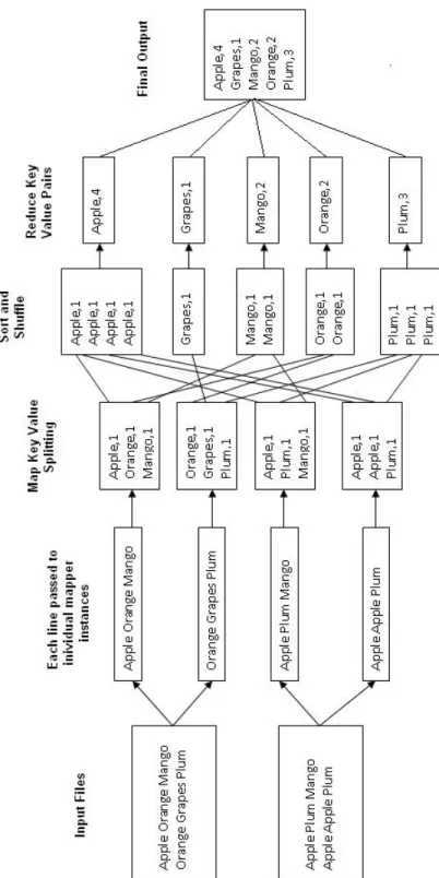
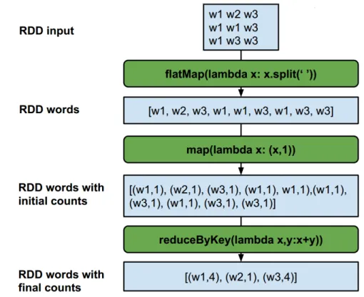
Fig. 2.7 shows the workflow of the MapReduce steps:

Splitting - it is a splitting criteria for the input data and it can be anything. comma, space or a new line and etc. Input data is divided into chunks depending upon the amount of data and capacity of units.

Mapping - mapper function start to work in this phase.

Intermediate splitting - this is a preparation for the reduce phase in order to group the data with similar KEY in the same cluster. The entire job process in parallel on different cluster.

Reduce - it is a group by phase, shuffling happens which leads to aggregation of similar patterns.

Combining - reducer combine the result set from each cluster to get the final result.

Most users find MapReduce attractive because of its simplicity, but there are some restrictions in this framework. Machine learning or graph algorithms require several iterations to process the data. Therefore, it is required to perform some computation on the same data. The computation in MapReduce starts with reading input data, processing it and then writing back to HDFS. In order to make the output ready as an input for the next job. The cycle of read, process and write had to be repeated till we get the result in iterative algorithms. However, it is costly for us to continuously do this expensive process. In iterative algorithms we want to read data once and iterate the data many times, MapReduce can not answer this needs in iterative algorithms. To overcome the these limitations of MapReduce, the Spark system [15] uses Resilient Distributed Datasets (RDDs) [15] which implements in-memory data structures that can keep the data across the set of nodes [36].

2.6

Spark

Based on the concept of Hadoop, Spark is a cluster computing framework that is developed in 2009 in UC Berkeley’s AMPLab. With Spark, processing of data become faster and easier [37]. Spark can be used in wide range of circumstances. Most of the scientists and application developers incorporate Spark into their applications to rapidly query, analyze, and transform data at scale. Interactive queries, processing of streaming data from sensors or financial systems, and ma-chine learning tasks can be implemented easily using Spark. It provides supports applications with working sets while providing similar scalability and fault toler-ance properties to MapReduce [36].

Spark is mainly developed and optimized to run in memory. As a result of that, it is faster than the Hadoop’s MapReduce, which tries to write and read data from computer hard drives between each stage of processing. Spark lets us to write application in Java, Scala [38], or Python languages. And, it facilitates working with it by interactively querying data within a shell. In addition to Map and Reduce operations, it supports SQL queries, streaming data, machine learning and graph data processing. In another word, Spark is a unified, comprehensive framework that big data with a variety of dataset nature (from test to graph data) and as well as different source of data (batch or real time streaming data) can be easily managed and processed.

2.6.1

Resilient Distributed Dataset

Resilient Distributed Dataset (RDD) is a core concept which is introduced by Spark, that is a fault-tolerant collection of elements that can be operated in parallel [15]. In another words, RDD is a read-only collection of objects that is distributed across a set of machine that if a partition of an RDD is lost, the RDD has enough information about how it was derived from other RDDs to be able to rebuild just that partition. [15]. RDD is a scalable and extensible internal data structure that enable in-memory computing and fault tolerance and these

features makes Spark as an inviting big data analytics tool in many industrial community.

RDD support two types of operations: Transformations and Actions. Transfor-mations create a new dataset from the existing one. Some of the Transformation functions are map, filter, flatMap, groupByKey, reduceByKey, aggregateByKey, pipe, and coalesce. And actions return a value to the driver program after run-ning the defined computation on the dataset. Some of the Action operations are reduce, collect, count, first, take, countByKey, and foreach. These operation provides convenience to the user to plug them on their own algorithms and apply them on RDD as algorithm frameworks in functional language style.

In this part we will examine word count implementation using Spark:

JavaRDD<String> textFile = sc.textFile("hdfs://..."); JavaPairRDD<String, Integer> counts = textFile

.flatMap(s -> Arrays.asList(s.split(" ")).iterator()) .mapToPair(word -> new Tuple2<>(word, 1))

.reduceByKey((a, b) -> a + b); counts.saveAsTextFile("hdfs://...");

In this example a few Transformations used in order to build a dataset of (String, Int) pairs called counts and then save it to a file

The data that is stored somewhere in HDFS is read into RDD of Strings called textFile. Each row of RDD consists of one line from the initial file. Now is the step to count the number of words:

1. RDD of lines transforms into RDD of words using flatMap RDD transfor-mation. flatMap is similar to a map in that it applies a function individually to each element in the RDD. But rather than returning a single element, it returns a sequence for each element in the list, and flattens the results into the one large result.

using map transformation. This will assign the value 1 to each of them.

3. Finally the aggregation happens and the values of similar keys are added to get the final word count using reduceByKey function. Fig. 2.6.1 represents the mentioned steps.

Figure 2.8: Workflow of the word count program using Spark.

M. Saravanan et al. proposed a distributed system based on MapReduce com-puting model for C4.5 decision tree algorithm [39] and performed extensive ex-periments on different dataset [40]. For privacy-preserving data sharing, they used perturbed data on decision tree algorithm for prediction. For private data analysis, they applied raw data to the privacy-preserving decision tree algorithm.

Chapter 3

Proposed Solution

In this section, our solution for privacy-preserving RIMARC algorithm is ex-plained in detail.

3.1

System and Threat Models

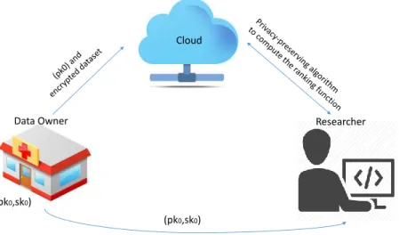
We have three main parties in the system: (i) data owner, who collects and provides the dataset that consists of sensitive data, (ii) cloud, which is responsible for the storage and processing of the dataset, and (iii) researcher, who is interested in analyzing the dataset and obtaining ranking functions out of it.

Dataset is stored in the cloud in encrypted form (details are provided in the next subsections). Our goal is to make sure that no party other than the data owner can access the plaintext (non-encrypted) format of the whole dataset. We also want to make sure that (i) the cloud does not learn any information about the dataset, including the result that is provided to the researcher, and (ii) the researcher only learns the results of his authorized query, and nothing else. In order to achieve these goals, we propose a privacy-preserving protocol between the cloud and the researcher in order to compute that AUC values. Our proposed protocol involves cryptographic primitives such as homomorphic encryption and

secure two-party computation.

We assume the data owner has the public/private key pairs (pko, sko) for the

Paillier cryptosystem (as discussed in Section 2.4). Public key of the data owner is known by all parties in the system and the secret key is only shared with the researcher (so that the researcher can decrypt and obtain the results of his queries). Note that, rather than providing the private key of the data owner to the researcher, it is also possible to use a threshold cryptography scheme, in which the private key is divided into two parts and these parts are distributed to the researcher and the cloud [41] . This threshold cryptography feature can be easily integrated into the proposed algorithm depending on the use case scenario. Our proposed system model is also illustrated in Fig. 3.1.

(pk0,sk0)

(pk0,sk0)

Data Owner Researcher Cloud

Figure 3.1: Proposed system model.

We assume that all parties in the system to be honest-but-curious. That

means that both the cloud and the researcher can try to access the sensitive data of the data owner (i.e., the content of the database), but they honestly follow the protocol steps. We also assume that the researcher and the cloud does not collude during the protocol. Of course, not every researcher can send queries to the dataset; the researcher should be authorized in order to do so. This can

be managed via an access control mechanism, which is out of the scope of this work. Finally, we assume all communications between the parties to be secured via end-to-end encryption.

3.2

Dataset Format and Encryption

Initially, the data owner collects data from the owners of the raw data records and constructs the dataset. For instance, this can be considered as a hospital collecting data from patients. We assume that the dataset consists of the records

of N individuals (e.g., N patients)1_{. The set of features in the dataset is illustrated}

as F = {f1, f2, . . . , fn} (we assume there are n features). Also, set of categories

for a given feature fi is represented as Ci = {c1i, c2i, . . . , cki}.

Here, we assume there are k categories per feature for simplicity, but each feature may also have different number of categories as well. Each category also

has a label `j<sub>i</sub>, where `j_i ∈ {0, 1}2_{, i ∈ F, and j ∈ C}

i.

We represent a category cj_i as below:

cj_i = bj,1_i ||b_ij,2|| . . . ||bj,j_i || . . . ||bj,k_i ,3

where bj,m_i = 0 when m 6= j and bj,m_i = 1 when m = j. For example, the

categories of color feature in our toy example (discussed in Section 2.3) and

their corresponding bit representations are illustrated in Fig. 2.4(b). In this

example, we have 5 categories (i.e., colors) for the color feature, and hence we use 5 bits in the representation, each assigned for a particular color. We use Paillier cryptosystem to encrypt the whole dataset.

In a nutshell, the data owner encrypts all categories and corresponding labels 1_{We also assume that continuous features are first discretized into categorical ones.}

2_`j

i = 0 represents a negative instance and ` j

i = 1 represents a positive instance. 3 _{|| represents the concatenation.}

using its public key (pko). To encrypt a category cji, the owner encrypts all its bits

individually. Thus, we represent the encryption of cj_i as [bj,1_i ]||[bj,2_i ]|| . . . ||[bj,,k_i ].4

The owner also encrypts all labels `j<sub>i</sub> to obtain the corresponding [`j_i] values. After

encryption, the data owner sends the encrypted data to the cloud for storage.

3.3

Privacy-Preserving RIMARC Algorithm

In this section, we will describe the privacy-preserving version of the RIMARC algorithm, that we call PP-RIMARC, in short.

The RIMARC algorithm learns scoring function and a weight for each feature. In the following, for the simplicity of the presentation, we describe the proposed

algorithm for a single feature fi with k categories. Note that the algorithm can be

easily generalized to handle multiple features, as we also show in our evaluations section. The main steps of the proposed solution are also illustrated in Fig. 3.2.

The scoring function for the feature fi is calculated using the equation 2.1, for

each category cj of the feature fi. It has a real value in [0,1]. Therefore, in order

to compute S(cj_i) P (cj_i), N (cj_i) have to be computed.

Initially, the cloud counts the number of instances of each category of the

feature fi in the dataset. To compute the total number of instances for the

category cj_i, the cloud computes P (cj_i) + N (cj_i) = [T (cj_i)] = PN

m=1[b m,j

i ]. This

summation can be easily carried out by using the homomorphic properties of the Paillier cryptosystem, as discussed in Section 2.4.

Then, the cloud counts the number of positive labelled instances for each

cat-egory. To do so, for each category cj_i, the cloud needs to compute [P (cj_i)] =

PN

m=1[b m,j

i ][`mi ]. This computation, however cannot be carried out by using the

homomorphic properties of the Paillier cryptosystem; as the homomorphic prop-erties do not support multiplication of two encrypted messages. Therefore, we 4_{In the rest of the paper, we use angled brackets to represent the encryption of a message} via Paillier encryption under the public key of the data owner.

1. Ask cl ou d to compu te the ran king fu nc tion for a giv en fea tur e tha t ha s k ca teg or ie s 2. Com pu te the tot al nu mbe r of in st an ce s of ea ch ca teg or y usin g the ho mom or ph ic pr op er ties of the Pai lli er cr yp tos ys tem 5. Compu te the sc or e val ue for ea ch ca teg or y usin g the secu re multip lic ation al gor ithm (Alg or ithm 1) 4. Compu te the tot al nu mber of ne ga tiv e la be lle d in st an ce s usin g the ho mom or ph ic pr op er ties of the Pai lli er cr yp tos ys tem 3. Comp ut e the tot al nu mber of po sitiv e la be lle d ins tan ce s using the secur e m ultip lic ation al gor ithm (Alg or ithm 1) 6. Sor t the compu ted sc or e val ue s usin g the secu re sortin g al gor ithm 7. Compu te the k+1 (F PR ,T PR ) po in ts usin g the ho mom or ph ic pr op er ties of the P ai lli er cr yp tos ys tem an d send the m to the resea rch er 8. Dec ryp t the rec ei ved po in ts and compu te the A UC

CL

OUD

RE

SE

AR

CHER

Figure 3.2: Overview of the proposed solution. Steps 3, 5, and 6 are interactive steps between the cloud and the researcher.

propose using the “secure multiplication algorithm”, in Algorithm 1 between the cloud and the researcher in order to handle this multiplication in a privacy-preserving way.

Algorithm 1 Secure Multiplication Algorithm

Input: @Cloud: encrypted messages [a] and [b]. @Researcher: (pko, sko). Output: @Cloud: [a × b]. @Reseacher: ⊥.

1: The cloud generates two random numbers r1 and r2 from the set {1,. . . ,K}. 2: The cloud masks [a] and [b]:

[ˆa] ← [a] × [−r1] = [a − r1], [ˆb] ← [b] × [−r2] = [b − r2].

3: The cloud sends [ˆa] and [ˆb] to the researcher.

4: The researcher decrypts [ˆa] and [ˆb] with sko: ˆ

a ← D([ˆa], sko), ˆ_{b ← D([ˆb], sko).}

5: The researcher computes ˆa × ˆb

6: The researcher encrypts the results with pko to get [ˆa × ˆb] and sends it to the cloud. 7: The cloud computes [a × b] ← [ˆa × ˆb] × [a]r2 _{× [b]}r1 _{× [−r}

1× r2].

We note that step 7 of Algorithm 1 is to remove the noise from the product and it can be easily done at the cloud using the homomorphic properties of the Paillier cryptosystem. We discuss the security of the secure multiplication algorithm in Section 3.4. Similarly, the cloud also computes the counts for number of negative

labelled instances for each category. To do so, for each category cj_i, the cloud

needs to compute [N (cj_i)] = [T (cj_i)] − [P (cj_i)]. Note that, this computation can

be easily handled at the cloud using the homomorphic properties of the Paillier cryptosystem. However, computation of counts for number of positive labelled instances and total number of instances is enough for calculating the score value.

Next, the cloud computes the score value for each category. As discussed

above, the encrypted score value for a category cj_i is computed as [S(cj_i)] =

[P (cj_i)]/[T (cj_i)]. Since Paillier cryptosystem does not support division of two

encrypted numbers, we propose normalizing the score value of each category. For this normalization, we compute the following normalization constant for each

[Z_ij] = k Y m=1 m6=j [T (cm_i )]. (3.1)

Since this computation requires multiplication of encrypted messages, we use the secure multiplication protocol in Algorithm 1, i.e., we iteratively multiply pairwise values. Then, the cloud computes the normalized score value for each

category cj_i as [ ˆS(cj_i)] = [P (cj_i)] × [Z_ij]. We emphasize here that we only need the

order relationship between the score values of categories to compute the AUC values. Therefore, this normalization does not affect the accuracy of the algo-rithm. The reason that the order of score values is preserved after normalization

is that we add the same constant [Z_ij] to each score values.

The computed normalized score values ([ ˆS(cj_i)]) need to be sorted in order

to compute the AUC values. This sorting operation can be securely carried on between the cloud and the researcher by using a “pairwise secure comparison al-gorithm” [42]. This interactive algorithm compares two encrypted numbers and returns an encrypted value (to the cloud) indicating which value is greater. How-ever, in our scenario, a feature may include tens of categories. Thus, such a pairwise comparison algorithm requires hundreds of pairwise comparisons, sig-nificantly reducing the efficiency of the algorithm. Therefore, for this step, we propose a more lightweight algorithm which only leaks the order of the normal-ized score values to the cloud. We describe this lightweight sorting algorithm in the following.

The cloud initially selects a random number r from the set {1, . . . , K} and

encrypts it via pko to get [r]. Then, for each normalized score value [ ˆS(cji)],

the cloud computes the masked score value [ ˜S(cj_i)] = [ ˆS(cj_i)] + [r]. Let g(.) be

a random shuffling function. The cloud shuffles the order of the masked score

values as g([ ˜S(c1

i)], [ ˜S(c2i)], . . . , [ ˜S(cki)]) and sends the masked (and encrypted)

score values to the researcher in the shuffled order. The researcher decrypts the

received score values using sko, and sorts them.

their masked order is the same as the unmasked one. Therefore, the researcher can compute the correct sorting of these values. After the values are sorted at the researcher, he/she only sends the sorted order of the masked score values back to the cloud. Using this information and the shuffling order of the score values (which is known by the cloud), the cloud obtains the sorted order of the score values of all categories. We briefly discuss the security of this sorting algorithm in Section 3.4.

The researcher only needs the k + 1 (FPR, TPR) points to generate the AUC

curve5. Knowing the order of [ ˆS(cj_i)] values, the cloud can easily compute the

k+1 encrypted ([FPR],[TPR]) points by using the number of positive and negative

labelled instances for each category (i.e., [P (cj_i)] and [N (cj_i)] values) and by using

the homomorphic properties of the Paillier cryptosystem (computation of the (FPR, TPR) points are discussed in Section 2.3). Finally, the cloud sends the k + 1 encrypted points to the researcher, the researcher decrypts the received

values by using sko, and constructs the AUC curve. Note that TPR is the fraction

of the true positives to the total positive labelled instances, and FPR is the

fraction of the false positives to the total negative labelled instances. Since,

this division cannot be carried out at the cloud, the cloud sends the numerator and denominator of each point to the researcher and the division is done at the researcher after the decryption.

3.4

Security Evaluation

Throughout the proposed algorithm, the cloud does not learn anything about the dataset of the data owner, and the researcher only learns the (FPR, TPR) points to generate the AUC curve.

The proposed algorithm preserves the privacy of data owner’s data relying on the security strength of the Paillier cryptosystem. The extensive security evalu-ation of the Paillier cryptosystem can be found in [23]. In particular, it is proved

that the cryptosystem provides one-wayness (based on the composite residuosity

class problem) and semantic security6 _{(based on the decisional composite}

residu-osity assumption).

We also use two interactive algorithms between the cloud and the researcher: (i) secure multiplication, and (ii) sorting. We briefly comment on their security in the following. During the secure multiplication algorithm, the cloud only gets

the encrypted multiplication value, and hence computes [P (cj_i)]. On the other

hand, the researcher (due to the masking with random numbers r1 and r2) cannot

observe any information about the labels or the categories.

During the sorting algorithm, since the values are masked and the researcher does not know the random number selected by the cloud, the researcher cannot learn the actual normalized score values. Furthermore, since the score values are shuffled at the cloud, the researcher cannot also learn which category has the highest score value. The cloud only learns the order of the normalized score values of the categories. Note that the data owner may prefer to keep the link between the bit encoding of a category and the name of the category hidden from the cloud (as the cloud does not need this information to do its operations). In such a scenario, learning the order relationship between the normalized score values does not mean anything to the cloud. Also, the selected random number r (from the set {0, . . . , K}) may be 0 with some probability. In this case, the researcher may learn the actual values of the normalized score values. However, this probability is negligibly small, especially for larger values of K.

3.5

Evaluation

In this section, we implement and evaluate the proposed algorithm on a real dataset. We used Wisconsin Diagnostic Breast Cancer (WDBC) dataset from UCI repository [43]. Dataset contains 569 individuals, each consisting of 31 fea-tures and labeled as either“M” for malignant (i.e., positive) and “B” for benign 6_{The adversary cannot distinguish between two different encryptions of the same message.}

Security Parameter n=512-bits Security Parameter n=1024-bits 16 Features 31 Features 16 Features 31 Features N=285

Individuals 9 minutes 17 minutes 56 minutes 106 minutes N=569

Individuals 19 minutes 26 minutes 97 minutes 187 minutes

Table 3.1: Time complexity of the proposed algorithm for different sizes of the security parameter (n), different number of features in the dataset, and different database sizes.

(i.e., negative). Also, each feature has different number of categories ranging from 8 to 19. As discussed, we used MAD2C algorithm for this step.

To evaluate the practicality of the proposed algorithm, we implemented it and assessed its storage requirement and computational complexity on Intel Core i5-2430M CPU with 2.40 GHz processor under Windows 7. Our implementation is in Java and it relies on the MySQL 5.5 database. We set the size of the security parameter n for the Paillier cryptosystem to 512 and 1024 bits in different experiments. In Table I, we summarize the time complexity of the proposed algorithm.

Based on the results, we can say that the time complexity of the algorithm increases linearly with the number of individuals and features. Total time to run the privacy-preserving algorithm is on the order of minutes. Furthermore, the proposed algorithm is highly parallelizable as computations on each feature can be carried out independently. We worked on the parallelization of the algo-rithm using Spark framework and we evaluated the performance of the proposed algorithm which is explained in the next chapter.

In terms of storage, the original (non-encrypted) dataset requires 120KB of storage space, while the encrypted version (thought the proposed algorithm) re-quires a disk space of 30MB when n = 512-bits and 60MB when n = 1024-bits.

This increase in the storage requirement is due to the ciphertext expansion of the Paillier encryption. There exists techniques to reduce this ciphertext expansion (such as packing [44]), and we will utilize these techniques to optimize the storage requirement in future work.

Note that non-private version of the algorithm runs on the order of seconds and requires less storage space. However, we believe that this increase in time and storage complexity is a reasonable compromise in order to obtain a privacy-preserving algorithm, which is a crucial requirement to process personal data

without privacy and legal concerns. We emphasize that the accuracy of the

results (i.e., obtained ranking function) for the private algorithm is exactly the same as the non-private version. To summarize, the performance numbers we obtained show the practicality of our privacy-preserving algorithm.