Temperature measurement and control circuit

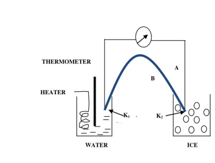
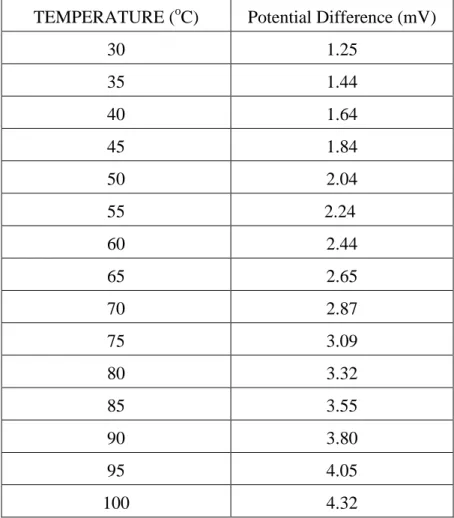
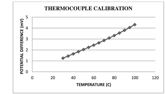
Thermocouples are a widely used type of temperature sensor for measurement and control and can also be used to convert a temperature gradient into electricity.. Commercial

As a result of long studies dealing with gases, a number of laws have been developed to explain their behavior.. Unaware of these laws or the equations

In each specific language similar words are represented differently not only quantitatively, but also qualitatively. In this paper, we analyze adjectives with a

In the methods we have applied so far in order to determine the relation between the atmospheric temperature and the pressure by using the annual average and amplitude

Şekil 6’daki düz çizgiler nokta etki-tepki tahminidir. Kesikli çizgiler ise bu tahminin %95 Hall güven aralığında olduğunu göstermektedir.. Şekil 5 ve 6'daki grafiklerin

Bulgular: Bilgisayar ve televizyon kullanım süresi ile uyku sorunu yaşama ve Beck Depresyon Ölçeği ortalamaları arasında bir ilişki bulunamamıştır (p>0.05).. Cep telefonunu

Süeda tanesi 20 kuruş olan kalemlerden 43 tane almıştır. Azra, Alihan' dan 9 yaş küçük olduğuna göre Azra kaç

Among patients whose body temperature values changed, the measu- red temperature values were divided into subgroups as being 36-37°C, 37-38°C, and >38°C in order to