THE APPLICATION OF STOCHASTIC PROCESSES IN CURRENCY EXCHANGE RATE
FORECASTING AND BENCHMARKING FOR USD-TL AND EURO-TL EXCHANGE RATES
GİRAY GÖZGÖR
1- CAHİT MEMİŞ
2- GÖKHAN KARABULUT
3Abstract
Since the first half of the 1990‘s many developing countries liberalizing their financial systems began to be more integrated to the global financial system. Due to the financial crisis, many developing countries have shifted to floating exchange rate regime. Thus, the significance of exchange rates has increased dramatically for the individual and institutional investors in the financial markets. Therefore, the number of studies which focus on forecasting the currency exchange rates increased dramatically. In this study, USD-TL and Euro-USD-TL exchange rate forecasts are generated via fundamental stochastic processes based on random walk or martingale, forward rates and the some time series models. The error performance values of the obtained results are tested via the test method developed by Diebold and Mariano (1995) and West (1996). It can be concluded that stochastic processes outperformed time series models for USD-TL exchange rates. According to the results stochastic process are generating more consistent and significant results. JEL Codes: C53, F31, G17.
Keyword: Exchange Rate Forecasting, Forecasting Performance, Stochastic Processes.
1
Introduction
After the collapse of the Bretton Woods System, the study of the estimation of floating exchange rates has been taking a steadily increasing share in the financial literature. Besides the structural-monetary modeling techniques of exchange rates based on different basic variables such as the gross domestic product, money supply, domestic interest rates, foreign interest rates and inflation and their differences, there are also various econometric techniques making use of time series.
Model using structural modeling techniques based on uncovered interest rates parity, law of one price and rational expectations theory enable the estimations. These models also include moving average (MA) and autoregressive (AR) regression processes. These kinds of models are widely used in the literature. The structural–monetary techniques and their accuracy have been studied by Hansen and Hodrick (1980), Wolff (1987), Taylor (1995), Mark and Choi (1997) and Mark and Sul (2001).
The most commonly used econometric techniques for exchange rate forecasting are ARIMA(p,d,q) models developed by Box and Jenkins (1970) and Var(p) models. Var(p) models are defined by Johansen and Juselius (1990) generalized using vector correction mechanisms (VECM) having n dimensions and p lags. The fundamental studies using time series models for exchange rates are those of Messe and Singleton (1982) who defined the unit root process, and Ahking and Miller (1987) who developed the theoretical structure enabling the application of stochastic processes and random-walk to exchange rate forecasts and compared with time series models.
Besides all these studies the fact that the spot values of exchange rates and their logarithmic returns follows a random walk was first been put forward by Mussa (1979). The studies arguing that random-walk and methods involving stochastic processes are defined based on random-walk assumption generate more significant results compared to the other methods mentioned.4 This idea can be traced back to the results put forward by Meese and Rogoff (1983a and 1983b). Meese and Rogoff (1983a and 1983b) compared structural models including monetary models, time series models and random-walk for exchange rate forecasts. They concluded that random-walk is the most significant forecaster. In these studies, Root Mean Squared Error (RMSE) method was used for comparison. The equations in Meese and Rogoff‘s approach were calculated using the time varying parameter models. Schinasi and Swamy (1989), on the other hand, indicated that time varying parameter models generate better results than random-walk when the Maximum Likelihood Estimator (MLE) technique in Kalman filtering method is used. Other studies indicating that random-walk is significant in the short and mid-term are Chinn and Meese (1995), Mark (1995) Marsh (2000), and Lyons (2002). On the other hand, Cheng, Chinn and Pascual (2005), concluded that none of the models or model types generates significant results in every case, thus for each different currency exchange rate a different model may be more effective.
Many authors explained the fact that random-walk models are more accurate exchange rate forecaster by referring to the existence of non-linearity in the data, which can not be explained by linear models such as time series models. Some of the studies indicating the non-linearity in the currency exchange rates include Hsieh (1988), Hsieh (1991), Hsieh (1993), and Hong and Lee (2003). In these studies the reason for non-linearity is explained through the non-existence of perfectly open economies in international trade. Dumas (1992) pointed to cost of carry, whereas Chinn (2001) tried to explain this phenomenon through menu costs.
Nevertheless, many different approaches were compared to random-walk models. Engel and Hamilton (1990) defined Markov Switching models for exchange rates and obtained much better results than random-walk. Similar but less significant results were also reached by Le Bron (1992) and Engel (1994). When these studies suggested that non-linear mean reversion may be used for currency exchange rates, Michael, Nobay and Peel (1997), Taylor and Peel (2000) and Taylor, Peel and Sarno (2001) suggested non-linear processes such as ESTAR models and new long-term regression processes. The study carried out by Killian and Taylor (2003) on these new methods indicates that these processes may generate more significant results. (But the recursive out-of-sample evidence does not reject random-walk forecast model). Similarly Neely and Sarno (2002) pointed to the accuracy of long-term regression processes and non-linear models. On the other hand, Hong, Li and Zhao (2007) indicated that random-walk models produce more
*
Dogus University, International Trade and Business, e-mail:[email protected] **
Risk Active, Specialist, e-mail:[email protected] *** Istanbul University, Economics, e-mail:[email protected] 1
The terms ‗random-walk‘ and ‗martingale‘ are interchangeably used in literature. However strictly speaking, the series are independent and identically distributed for ‗random-walk‘ while there is a martingale difference sequence for ‗martingale‘.
accurate results than most time series, non-linear models and Markov Switching models. Yang, Su and Kalori (2008) investigated the Martingale behavior of seven major Euro exchange rates using out-of-sample forecasts. In their study, Diebold and Mariano (1995) and West (1996) test statistics failed to reject the Martingale hypothesis for all seven Euro exchange rates. Hence with their new criteria, they found little evidence against the martingale behavior for the three major Euro exchange rates which is useful in providing evidence of nominal exchange rate predictability.
This study aims to analyze the free market Euro-TL and USD-TL daily exchange rate and their yield changes between January 2007 and January 2009 and to compare forecast results. The monthly, three-monthly and six-monthly forecast performances of five different stochastic processes (Geometric Brownian Motion, Discrete Brownian Motion, Generalized Wiener, Ito, Mean Reverting) and Var(p), ARIMA (p,d,q), UIP (forward rate) were compared for the mentioned time period. Subsequently the error values of the exchange rate forecasts were calculated according to performance criteria and this error values are compared with the test statistics proposed by Diebold and Mariano (1995) and West (1996). Our study will be first paper to apply stochastic models in forecasting exchange rates to Turkey Exchange Rate Markets
Firstly, the method and assumptions of this study and the models used for the mentioned time period will be defined. Then, volatility term and random term of the stochastic processes will be assessed and the exchange rates and forecast error rates will be calculated. In the last section the error values will be subject to comparison.
2
Data and Methodology
This study is based on the daily 1620 free market closing data, date 2002:03-2009:01. The reason underlying the choice of this time period is the fact that in this time period the floating exchange rate regime took effect in Turkish foreign currency exchange market. The mentioned exchange rate values are obtained from Bloomberg. However, the time period mentioned is only been used for the time series methods. In order to generate more effective results in forecasting the random and volatility terms of stochastic processes, a shorter period is used, the reason of which will be discussed later in detail.
The shorter time periods used for stochastic processes also applied to the time series approach and the exchange rate values with least error are chosen to generate the estimations of the corresponding model. The shorter time period used for comparison is January 2007-January 2009.
The stochastic processes used in this study are generated via Java and SQL based algorithms. Accordingly, the stochastic process has three parts. These are the mean average part based on past yields, the variance part based on volatility values and the random part based on distributions. At this point, the stochastic processes estimated one single day by dividing it into 100 parts (path=100) and using 1000 different simulations (n=1000). The estimated exchange rate value for that day is the arithmetic mean of all the values calculated according to this method. At this point, it is important to note that the simulation results are strictly based on the arithmetic mean and no correction to random processes has been made to increase the accuracy of the models– not even for the periods of crisis with extreme values.
The probability distributions used in the analysis to define the random parts of the stochastic processes are examined according to Pearson‘s Chi-Square and Kolmogorov-Smirnov (K-S) test criteria and through a rolling window approach the distributions appropriate for the yield values of the last 500 days (2years) are used. Accordingly, the probability distributions are chose n from distributions that are able to produce negative and positive changes in rates of return, random negative results and extreme values if necessary. At this point, the process of random number production strictly sticks to the parameter values calculated through the probability distributions. Moreover, the random numbers obtained are fixed for each day since the performances of the stochastic processes will be compared for each day and the same random numbers are used for all the processes. Hence, the changes in distributions and/or parameters according to the mentioned test criteria for each day have been reflected to all the stochastic processes as such.
Nevertheless, volatility values of the variance part in the stochastic models are estimated using the GARCH (1,1) model. The reason to choose the GARCH (1,1) model to estimate the volatility is the study conducted by Hansen and Lunde (2005) showing t hat the GARCH (1,1) model is more accurate than various other volatility models. In this study, in a comparison among 330 ARCH type models, they find no evidence that a GARCH (1,1) model has been outperformed in their analysis of exchange rates. Additionally, Engel and Ng (1993) suggest that asymmetric volatility models (EGARCH, GJR, QGARCH among others) were not considered given that they are not theoretically justifiable for exchange rate modeling. This is because there is no proven statistical evidence that exchange rate volatilities have asymmetric volatility. In fact, no asymmetrical volatility is found for the data considered in this study. To test for asymmetric volatility the method suggested by Engel and Ng (1993) was employed. The details of the tests necessar y for the GARCH (1,1) models will be explained in the application chapter.
In this study, besides the five stochastic processes (Geometric Brownian Motion, Discrete Brownian Motion, Generalized Wiener, Ito, Mean Reverting) Var(p), ARIMA (p,d,q) and UIP (forward rate) models are used. For Var(p) and ARIMA (p,d,q) the most accurate forecaster producing model is generated via Bayesian information criteria and Akaike information criteria. It is important to note that in comparison to the values obtained by time series approach, a dynamic (rolling window) forecast is carried out as has been calculated for the stochastic processes.
The risk-free interest rates used for the foreign currencies in the uncovered interest rate parity (forward rate) model are the arithmetic mean of 30, 60 and 90 day returns on the daily yield curve of the benchmark bonds in the Turkish Bond Market for the corresponding period of this study and are calculated according to the Nelson and Siegel (1987) method. The data for these calculations are obtained from Bloomberg. When there are no transactions in the markets from where the data was obtained but the Turkey Market was active, the data of the previous day is used.
Firstly, the properties of the probability distributions will be briefly explained and the GARCH (1,1) process will be defined. Then, the test to estimate the volatility will be carried out and the volatility values for each day will be found. After the stochastic processes, the time series models and UIP models are explained, in the application part all the exchange rate values will be calculated through these models. Finally, the results will be compared to assess the forecast performances of the models.
2.1
The Probability Distributions
The probability distributions mentioned below constitute the randomly developing part of the exchange rate estimation and the stochastic processes in the determination of exchange rate volatility calculated according to the Anderson and Darling (A-D) and Kolmogorov-Smirnov (K-S) statistics on the basis of yields of the relevant period.
Normal Distribution, If real-valued random X variable XЄ(-∞,∞), µ is the mean and ζ2 is the variance, the equation is
X~N(µ, ζ2) pdf = 2 2 1 ( ) exp( ) 2 2 x
cdf = 1 (1 ( )) 2 2 x erf
mgf= exp( 2 2) 2 t t
Student-t Distribution, For the real-valued random and the independent X variable XЄ(-∞,∞), let v be the degree of freedom, µ is
the population mean and
is the gamma function, then X~GH(-
/2, 0, 0, , ,µ) pdf=1 2 ( ) 2 1 ( ) 2 (1 ) ( ) 2 v v x v v
cdf = 2 2 1 1 11 3 ( ( 1)) (; ( 1); ; ) 1 2 22 2 1 2 ( ) 2 t t v F v v v v
mgf is not defined here.
Hyperbolic Secant Distribution, Compared to a standard normal distribution it is a leptokurtic distribution. For countries having leptokurtic distribution problems such as Turkey it has become important. For XЄ(-∞,∞) sech( ) 2
x x x e e is calculated for pdf = 1 sec ( ) 2 h 2x cdf = 2 arctan[exp( )] 2x mgf=t 2 sec( )t
Logistic Distribution, For real-valued random independent X variables, when XЄ(-∞,∞) , µ is the mean and s is the standard
deviation, then ( ) 1 e Z e
and if 1 1 1 0 ( , ) x (1 )y B x y
t t dtRe( ), Re( )
x
y
0
pdf = ( ) / ( ) / 2 (1 ) x s x s e s e and cdf = ( ) /1
1
e
x s mgf=st
1
t (1 ,1 ) e B st stLog-Logistic Distribution, For real-valued random independent X variables, when XЄ,
(
>0) is the median,
(
>0) is the Beta functionb
, E(x) = sin b b
(for
>1), the variance is V(x)= 22 2 2 ( ) sin 2 sin b b b b (for
>2) pdf = 1 2 ( / )( / ) [1 ( / ) ] x x cdf = 1 1 ( / ) x Moment generating function (mgf) is not defined here.
2.2
Volatility
For the volatility estimation, GARCH(p,q) models are used. GARCH(p,q) models have been put forward by Engle (1982) and then developed and generalized by Bollersev (1986). These models include the martingale approach indicating the lack of relation between stochastic processes of the rate of returns and the stochastic realizations but also noting that they are not totally independent of each other. The formula for the GARCH (1,1) is as follows Bollersev (1986) and Taylor (1986). The first equation is:
2 1 1 . . ., ( ) 0, ( ) 1 t t t t t t t t t r u z z i i d E z Var z
Where
r
t is the return at time t, calculated as the logarithmic difference of the exchange rate, i.e. rt pt pt1wherep
is thenatural logarithm of the exchange rate,
u
t t1 is the conditional variance andz
t denotes a mean zero, variance one, serially uncorrelated error process. The GARCH(1,1) model for the conditional variance is:2 2 2
1
1 t 1 2
t t t t
(1)The condition for this is 0, 0,0 In order for the variance to be stationary in the GARCH(p,q) process it is assumed that
1 1 1 p q i j i j
. It is also assumed that in the GARCH(1,1) model, there is no autocorrelation but randomness at the square of the expected errors in the forecasted yield variables.At this point, it is important to note that the autocorrelation analysis of the Usd-TL and the Euro-TL exchange rate values has been carried out while calculating volatility in the GARCH (1,1) model. If the probability (p) value is greater than 0,01, it means that there is no autocorrelation. And the fact that there is no autocorrelation means that the GARCH(p,q) models generate consistent forecasts. At this point, 15 is used as the lag value as suggested by Engel (2001). Accordingly, if the p values are greater than 0,01 , there is no autocorrelation among the standardized error terms of the time series. Hansen and Lunde (2005) show that the GARCH(1,1) model generates consistent and significant results up until 500 observations for a time series with no autocorrelation and which estimates the conditional variance correctly. Over 500 observation values, however, asymmetric models based on more
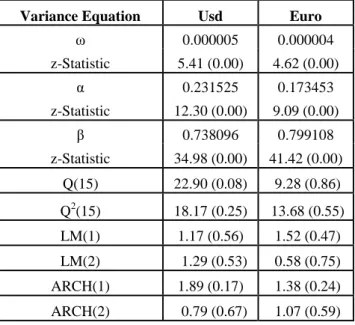
sensitive measures are required. Since the forecasting period in this study covers 504 observations5 and there is no autocorrelation, models are expected to generate consistent results. In order to show that autocorrelation results Q and LM tests might be used. At the same time in order to show the accuracy of specification of the variance equation Q2 statistics and to show the ARCH effect of the lags in variance equations ARCH tests might be used. In order to determine that the GARCH (p,q) model is appropriated, AIC and BIC have been used.
Table 1: GARCH(1,1) Model Parameters and the Autocorrelation Test Results Variance Equation Usd Euro
ω 0.000005 0.000004 z-Statistic 5.41 (0.00) 4.62 (0.00) α 0.231525 0.173453 z-Statistic 12.30 (0.00) 9.09 (0.00) β 0.738096 0.799108 z-Statistic 34.98 (0.00) 41.42 (0.00) Q(15) 22.90 (0.08) 9.28 (0.86) Q2(15) 18.17 (0.25) 13.68 (0.55) LM(1) 1.17 (0.56) 1.52 (0.47) LM(2) 1.29 (0.53) 0.58 (0.75) ARCH(1) 1.89 (0.17) 1.38 (0.24) ARCH(2) 0.79 (0.67) 1.07 (0.59)
Graph 1: USD-TL Daily Return Graph
Graph 2: Euro-TL Daily Return Graph
Among the currency values obtained the extreme values are accepted as calculated and they are not processed further. As seen on the graph, USD-TL and Euro-TL series are stationary. Moreover, the unit root tests suggested by Kwiatkowski et al. (1992) and Phillips and Perron (1988) for the mentioned series are tested and it is proved that they are stationary. Since the volatility values for the corresponding days are required to make a comparison, the obtained results are not also included in the study.
2
Since the forecasts start from January 2007, in GARCH (1,1) model for the last 504 observations beginning from January 2005 the rolling window approach has been applied.
As is mentioned by Johnston and Scott (2000) on the basis of these test results the GARCH (1,1) model is used to calculate daily volatility values of exchange rates.
2.3
Stochastic Processes
Stochastic processes used in this study are the Geometric Brownian Motion, Discrete Brownian Motion, Generalized Wiener process, Ito stochastic process, and the Mean Reverting (Ornstein-Uhlenbeck) process. These stochastic processes show either Martingale or Markov process properties. In the Markov process the changes in every period are independent from each other. The Martingale approach, on the other hand, claims that there is no correlation between stochastic processes and stochastic realizations but they are not totally independent. According to Duffie and Glynn, (2004) if a distribution has ( , , ) parameters
X t
t0 and ifthe stochastic process is defined as
t t0and if
X t
, ( )t
t0; Xt
, t
0and Xt
s Xs
0 s t, then it can be said that the stochastic process shows martingale properties. And if
0 , ( ) t X t t ;
X t
B
s
X t
B X s( )
0 s t,
B , then the mentioned stochastic process is considered to show the properties of the Markov process. In order to make assumptions it is important to determine whether the stochastic processes show properties of the martingale or the Markov process. So that the use of stochastic processes in exchange rate forecasting becomes possible.
Accordingly, if a St – valued asset follows a stochastic process as is shown below, it is called the Geometric Brownian Motion: given that dStS dtt S dWt t, let Wtbe the Wiener process,
denotes the percentage drift and
shows the percentage volatility.When the equation is solved the process is defined as 2
0 1 exp(( ) ) 2 t t S S tW .
Discrete Brownian Motion, If any of the above mentioned distributions have the ( , , ) parameters, given that k=0,1,2….N and
assuming that a filtering system as { }k is used, Yi~N(0,1) shows independent standard normal distribution parameters and let B0=0 be the initial point and given that Bk=
1 k i i Y
, k=1,…N Bk~N(0,k) , then{ }
k 0 N kB
is defined as such. In Discrete Brownian motionevery change shows independent and standard normal distribution and it shows properties of the martingale and the Markov
processes. Accordingly the discrete Brownian motion is defined as such: 2
0 1 exp( ( ) ) 2 k k S S B k k=0,1,2…N.
Generalized Wiener process given thata x t dt( , ) b x t( , ) dt where a and b are indicated deterministic function, t is time, x is underlying asset, dt is the differential equation can be related to Wiener process,
is random numbers which are obtained randomly by relevant distributions.Ito stochastic process given that dSt tdBttdtwhere St value of asset, Bt is any random process,
is drift
is volatility.Ito‘s Lemma formula derivated from Ito Process and defined such as ( , ) ( 1 2 2) 2 h h h dh t W dW t W W
whereby Wiener process.
Mean Reverting (Ornstein-Uhlenbeck) Process, if a St – valued quantity follows a stochastic process as is shown below, it is called the mean reverting process: given that dSt ( S dtt) dWt
>0 ve,
>0; Wt denotes the Wiener process, showsthe percentage of drift and let
be the percentage of volatility and if the equation is solved based on the assumption that W definesthe Wiener process, then the process can be defined as such: 2
0 (1 ) ( 1) 2 t t t t t S S e e W e e
In order to solve the equations in the above mentioned processes the approach suggested by Smith (1991) is followed. Accordingly, by using one of the mentioned processes and given that path=100 n=1000 a sample algorithm of Geometric Brownian Motion process showing single-day Euro-TL parity can be showed as such:
In this way, univariate modeling is done through the Box-Jenkins type ARIMA(p,d,q) modeling where lag selection is done via AIC and BIC and ensuring there is no pattern left in the residuals. Exchange rate depreciation, that is the first difference of the natural logarithm of the exchange rate, is modeled by the equation
0 1 1 2 2 ... t t t t S S S where t S
shows the first difference of the natural logarithm of the exchange rate at time t, and
t is a white noise error term. In addition, multivariate time series modeling is applied through an unconstrained VAR(p) as0 1 1 2 2 ...
t t t t
X X X E
whereXt is an (nx1) vector of endogenous variables which may include the domestic interest rate as well as the exchange rate, and Et is a vector of white noise error terms. The reason for estimating such a VAR(p) is to see how the dynamics of the interest rate as well as the exchange rate itself might have an impact on the exchange rate and hence might have an added value for forecasting the future values of the exchange rate. Note that as the data frequency is daily, there is an ARCH effect in the data and hence volatility modeling is done.
The basic uncovered interest parity (UIP) condition expresses the expected depreciation as a function of the interest differential and under the assumptions that the foreign exchange market participants are risk neutral, and the underlying alternative domestic and foreign assets are perfect substitutes states that the expected depreciation of the domestic currency against the foreign currency over k periods is equal to the premium of the return on the domestic asset over that on the foreign asset, both with time to maturity of k periods. The UIP condition is defined as
* 0 1 ( ) t k t t t t k S S i i where t
S denotes the natural logarithm of the nominal exchange rate expressed as the amount of domestic currency per unit of
foreign currency, k is the investment horizon i , and t
i
t* are k-period domestic and foreign interest rates, respectively and
is takenas the rational expectations forecast error.
3
Evaluation of the Forecasts and Empirical Findings
This study is based on forecasts in three different time periods. For monthly, three-monthly and six-monthly forecasts the method of Meese and Rogoff (1983a) was followed. At this point, via the rolling window estimation model initially n observations (n=504) are used and then monthly three-monthly and six-monthly forecast are made. Let T be the number of total observations, then sequential (T-n) was used for forecasting. The forecasts obtained were compared to the actual values and the differences constitute the expectation of forecast errors. This process applied to all methods and the out-of-sample forecasts were compared.
Meese and Rogoff (1983a) is based on random walk as the benchmark model, whereas this study is based on ARIMA (p,d,q) model.
Statistics of expectation forecast errors are used for comparison of forecast rates with realized values regardless of the differences in sign and scale. The most commonly used statistics of expectation forecast errors are the root mean square error (RMSE), the mean absolute error (MAE), mean absolute percentage error (MAPE) and the Theil-U factor. In a comparison of forecast models, the lower RMSE, MAE, MAPE and Theil-U values indicate more accurate models. According to Poon (2005) expectation forecast error statistics are defined as such:
RMSE= 2 2 1 1 1 1 ˆ ( ) N N t t t t t N
N
MAE= 1 1 1N 1Nˆ t t t t t N
N
MAPE= 1 1 ˆ 1N 1N t t t t t t t N N
Accordingly the error statistics for exchange rates are shown in the table:
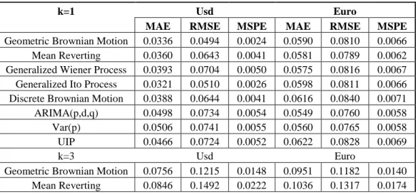
Table 2: Error statistics for USD-TL and Euro-TL
k=1 Usd Euro
MAE RMSE MSPE MAE RMSE MSPE
Geometric Brownian Motion 0.0336 0.0494 0.0024 0.0590 0.0810 0.0066
Mean Reverting 0.0360 0.0643 0.0041 0.0581 0.0789 0.0062
Generalized Wiener Process 0.0393 0.0704 0.0050 0.0575 0.0816 0.0067
Generalized Ito Process 0.0321 0.0510 0.0026 0.0598 0.0811 0.0066
Discrete Brownian Motion 0.0388 0.0644 0.0041 0.0616 0.0840 0.0071
ARIMA(p,d,q) 0.0498 0.0734 0.0054 0.0549 0.0760 0.0058
Var(p) 0.0506 0.0741 0.0055 0.0560 0.0765 0.0058
UIP 0.0466 0.0724 0.0052 0.0622 0.0828 0.0069
k=3 Usd Euro
Geometric Brownian Motion 0.0756 0.1215 0.0148 0.0951 0.1182 0.0140
Generalized Wiener Process 0.0900 0.1582 0.0250 0.1191 0.1418 0.0201
Generalized Ito Process 0.0806 0.1296 0.0168 0.1002 0.1249 0.0156
Discrete Brownian Motion 0.0890 0.1609 0.0259 0.1161 0.1388 0.0193
ARIMA(p,d,q) 0.1183 0.1598 0.0255 0.1175 0.1404 0.0197
Var(p) 0.0990 0.1567 0.0245 0.0928 0.1231 0.0151
UIP 0.1162 0.1583 0.0251 0.1218 0.1448 0.0210
k=6 Usd Euro
Geometric Brownian Motion 0.1364 0.1713 0.0294 0.1262 0.1700 0.0289
Mean Reverting 0.1619 0.1959 0.0384 0.1320 0.1357 0.0184
Generalized Wiener Process 0.1682 0.2193 0.0481 0.1465 0.1707 0.0291
Generalized Ito Process 0.1439 0.1812 0.0328 0.1317 0.1756 0.0308
Discrete Brownian Motion 0.1599 0.2084 0.0434 0.1589 0.1833 0.0336
ARIMA(p,d,q) 0.1768 0.1911 0.0365 0.1264 0.1449 0.0210
Var(p) 0.1618 0.1988 0.0395 0.1309 0.1362 0.0186
UIP 0.1810 0.2078 0.0432 0.1255 0.1625 0.0264
At this point, the Diebold and Mariano and West (DMW) test, which is used to test whether there is significant difference between the mentioned forecast errors, is defined as such:
H0: 2 2 1 2
0
H1: 2 2 1 20
( 2 2 1 2 0 or 2 2 1 2 0 )According to this test one model is considered to be fixed. In our study this model is the ARIMA (p,d,q) model. Accordingly the model‘s MSPE values are calculated as such
2 1 2
1 P (yt i)
. (2)On the other hand, the MPSE value of the other model subject to comparison with the fixed model is calculated as such:
2 1 2
2 P (yt i yˆt i)
(3)It is important to note that yt i denotes the standard deviation of the fixed model, whereas yt i yˆt i shows the deviation of the
model subject to comparison. P is the number of observations.
Diebold ve Mariano (1995) and West (1996) developed the t-test to compare the performances of the fixed model with other models. According to this, while the null hypothesis value shows that the performances of both of these models are equal, an alternative hypothesis shows that the other models are less accurate than the fixed model because they contain more errors and therefore have lower forecasting value.
Accordingly, the DMW test statistic is defined as such:
1 f DMW P V (4) ˆ ( ) t i t i t i f y y y (5) 1 f P
f and VP1
( )f 2 (6)Accordingly, the DMW test results calculated for forecast methods are as shown in appendix. According to the results of this test between the different exchange rates calculated through different forecasting methods for USD-TL, monthly forecasts generated by Mean Reverting and Ito process have %5 significant differences. For three-monthly USD-TL forecasts generated by Mean Reverting and Ito Process the significance level is %1, for six-monthly forecasts, on the other hand the significance level is %5. It can be said that the Geometric Brownian Motion generates more accurate forecasts than the other methods. For Euro-TL, however, the monthly and six-monthly forecasts do not have significant differences and for three-monthly forecasts Var(p) model generated results at %1 significance level and are more accurate than the other models. At this point, a more general evaluation of the effectiveness of the models show that none of the models are prominent for Euro-TL in monthly, three-monthly and six-monthly periods, whereas Ito process and/or Geometric Brownian Motion processes can generate more accurate results for USD-TL currency exchange rates.
4
Conclusion
Due to the invention of financial models and instruments/products for following developments in financial information and technologies, the predictability of exchange rates has become more complicated. Over the time, forecasting methods transformed from linear models to more dynamic structures. During this transformation process the developments in both time series models and random walk-martingale models led to advancements in exchange rate forecasts. The continuous growth in the number of models has caused institutions and investors trying to secure accurate pricing and forecasting to compare the performance of different models.
The literature on exchange rate predictions is extensive. There are many different models and systems for prediction and comparative studies on their performances. Thus, the available information on the subject increases constantly. However, one of the most crucial factors affecting the accuracy of predictions is the application of the right information and the right model at the right time. Looking at price data of exchange rate predictions to remove the information differentiation does not provide the neces sary information to evaluate effectiveness. In order to achieve accuracy of the model, the ‗performance measurements‘ should be checked and the results should be compared to these measurements frequently.
In this study, besides the prediction of currency exchange rates through time series models, stochastic processes and forward rates, the error performances of these values are calculated and the significance tests are performed. These predictions have a dynamic structure and are calculated based on different probability distributions or parameters at every observed value using the GARCH (1,1) model for volatility. Since the period was marked by volatility shocks, in order to show the reliability of statistical methods and forecast performance, the results should not be expected to be the same every time. In time, the probability distribution of the currency exchange rate, the volatility structure and jump feature can change; therefore the analysis should be assessed in the corresponding period.
After looking at the error performance tests, the study concludes that the most accurate model of USD-TL exchange rate for one-three and six months is the Geometric Brownian Motion model. On the other hand, the error performance of the stochastic models for the USD-TL exchange rates are more accurate compared to time series models and forward exchange rate with the exception of forecasting three months Var(p) model. In addition to the Geometric Brownian Motion model, the results of the Ito Process sho w significant differences for the USD-TL exchange rate for each forecasting period. Thus it can be said that it is also accurate model. It can also be concluded that different models are more significant and accurate for different periods.
For the Euro-TL exchange rate, none of the model groups are significantly different. Nevertheless, in the long run the Mean Reverting Model and in the short run the ARIMA (p,d,q) and Var(p) model are well performed according to performance values. However, the results we obtained do not indicate which models should be used in which periods. The Euro-TL exchange rate forecast showed that it rapidly changes in time and therefore this forecasting requires to be modeled differently. The lack of accurate modeling arose from the parity effect of the USD-Euro exchange rate in the period in question. Accordingly, none of the models were sufficient to show this parity effect. According to Diebold and Mariano (1995) and West (1996) tests there is no significant difference. This indicates that the parity effect on the prediction of the Euro-TL exchange rate has to be additionally modeled with volatility models used in stochastic models or with distribution parameters. This point might be subject of further study.
The reliability of predictions of currency exchange rates and the accuracy of the models has been the subject to long lasting debate. In addition to the accuracy of the forecasts, models should also have consistency over a length of time. Over time, the application of the sound models might give information about their suitability to the changing volatility of exchange rate premiums and to the probability distribution; however this information does not provide a definite conclusion for the accuracy of the model. Therefore, it is important to note that in exchange rate forecasting not all models will be effective in every market condition. Even if the model has been well-performed in the associated period, the most significant criterion for well-performed forecasting is that the model needs to be adapted over time to different probability distributions according to market conditions or to volatility models.
5
References
Ahking, F.W.-Miller, S.M. (1987), ‗Comparison of the Stochastic Processes of Structural and Time-Series Exchange-Rate Models‘, The Review of Economics and Statistics, 69:496-502.
Bollersev, T. (1986), ‗Generalized Autoregressive Conditional Heteroskedasticity‘, Journal of Econometrics, 31:307-328. Box, G.E.P.-Jenkins, G.M. (1970), Time Series Analysis, Forecasting and Control, Holden-Day: San Francisco, CA.
Cheung, Y.W.-Chinn, M.D.-Pascual, A.C. (2005), ‗Empirical Exchange Rate Models of the Nineties: Are Any Fit to Survive?‘ Journal of International Money and Finance, 24:1150-1175.
Chinn, M.-Richard, M. (1995), ‗Banking on Currency Forecast: How Predictable is Change in Money?‘ Journal of International Economics, 38:161-178.
Chinn, M. (2001), ‗Menu Costs and Nonlinear Reversion to Purchasing Power Parity among Developed Countries‘, UCSC Dept. of Economics Working Paper, 498.
Dumas, B. (1992), ‗Dynamic Equilibrium and the Real Exchange Rate in a Spatially Separated World,‘ Review of Financial Studies, 5:153–180.
Diebold, F.X.-Mariano, R.S. (1995), ‗Comparing Predictive Accuracy‘, Journal of Business and Economic Statistics, 13:253-263. Duffie, D.-Glynn, P. (2004), ‗Estimation of Continuous-Time Markov Processes Sampled at Random Time Intervals‘, Econometrica, 72:1773-1808.
Engel, C.-Hamilton, J.D. (1990), ‗Long Swings in the Exchange Rate: Are They in the Data and Do Markets Know It?‘ American Economic Review, 80:689-713.
Engel, C. (1994), ‗Can the Market Switching Model Forecast Exchange Rates‘, Journal of International Economics, 36:151-165. Engle, R.F. (1982), ‗Autoregressive Conditional Heteroskedasticity with Estimates of the Variance of United Kingdom Inflation‘, Econometrica, 50:987–1007.
Engle, R.F. (2001), ‗The Use of ARCH/GARCH Models in Applied Econometrics‘, Journal of Economic Perspective, 15:157-68. Engle, R.F.-Ng, V.K. (1993), ‗Measuring and Testing the Impact of News on Volatility‘, Journal of Finance, 48:1749-1778. Hansen, L.P-Hodrick, R.J. (1980), ‗Forward Exchange Rates as Optimal Predictors of Future Spot Rates: An Econometric Analysis,‘ Journal of Political Economy, 88,:829-853.
Hansen, P.R.-Lunde, A. (2005), ‗A Forecast Comparison of Volatility Models: Does Anything Beat A GARCH (1,1)?‘ Journal of Applied Econometrics, 20: 873-889.
Hong, Y.M.-Lee, T.H. (2003), ‗Inference on Predictability of Foreign Exchange Rates via Generalized Spectrum and Nonlinear Time Series Models‘, Review of Economics and Statistics, 85:1048-1062.
Hong, Y.M.-Li, H.-Zhao, F. (2007), ‗Can The Random Walk Model Be Beaten in Out of Sample Density Forecasts? Evidence from Intraday Foreign Exchange Rates‘, Journal of Econometrics, 141:736-746.
Hsieh, D.A. (1991), ‗Chaos and Nonlinear Dynamics: Application to Financial Markets‘, The Journal of Finance, 46:1839-1877. Hsieh, D.A. (1993), ‗Implications of Nonlinear Dynamics for Financial Risk Management‘, The Journal of Financial and Quantitative Analysis, 28:41- 64.
Hsieh, D.A. (1988), ‗The Statistical Properties of Daily Foreign Exchange Rates: 1974-1983.‘, Journal of International Economics, 24:129-145.
Johansen, S.-Juselius K. (1990), ‗Maximum Likelihood Estimation and Inference on Cointegration – with Applications to the Demand for Money,‘ Oxford Bulletin of Economics and Statistics, 52:169-210.
Johnston, K.-Scott, E. (2000), ‗GARCH Models and The Stochastic Process Underlying Exchange Rate Price Changes‘, Journal of Financial and Strategic Decisions, 13:13-24.
Kilian, L.–Taylor, M.P. (2003), ‗Why Is It So Difficult to Beat the Random Walk Forecast of Exchange Rates?‘ Journal of International Economics, 60:85-107.
Kwiatkowski, D.-Phillips, P.C.B.-Schmidt, P.-Shin, Y. (1992), ‗Testing the Null Hypothesis of Stationarity against the Alternative of a Unit Root‘, Journal of Econometrics, 54:59–178.
Le Baron, B. (1992), ‗Forecast Improvements Using A Volatility Index‘, Journal of Econometric Applications, 7:137-149. Lyons, R.K. (2002), ‗Foreign Exchange: Macro Puzzles, Micro Tools‘, Economic Review Federal Reserve Bank of San Francisco, 1:51-69.
Mark, N.C. (1995). ‗Exchange Rates and Fundamentals: Evidence on Long-Horizon Predictability‘ American Economic Review, 85: 201-218.
Mark, N.C.-Choi, D.Y. (1995), ‗Real Exchange Rate Prediction over Long-Horizon‘, Journal of International Economics, 43:29-60.
Mark, N.C.-.Sul, D. (2001), ‗Nominal Exchange Rates and Monetary Fundamentals: Evidence from a Small Post Bretton-Woods Panel‘, Journal of International Economics, 14:3-24.
Marsh, I.W. (2000), ‗High Frequency Markov Switching Models in the Foreign Exchange Rate Market‘, Journal of Forecasting, 19:123-134.
Meese, R.A-Singleton, K.J. (1982), ‗On Unit Roots and the Empirical Modeling of Exchange Rates‘, The Journal of Finance, 37:1029-1035.
Meese, R.A.-Rogoff, K.S. (1983a), ‗Empirical Exchange Rate Models of the Seventies: Do They Fit Out of Sample?‘, Journal of International Economics, 14:3–24.
Meese, R.A.-Rogoff, K.S. (1983b), The Out of Sample Failure of Empirical Exchange Models In Exchange Rates and International Macroeconomics, edited by Jacob A. Frenkel. Chicago Univ. Press: Chicago.
Michael, P.-Nobay, R.A-Peel, D.A. (1997), ‗Transaction Cost and Nonlinear Adjustment in Real Exchange Rates: An Empirical Investigation‘, Journal of Political Economy, 105:.862-879.
Mussa, M.L. (1979), ‗Empirical Regularities in the Behavior of Exchange Rates and Theories of the Foreign Exchange Market‘, Carnegie- Rochester Series on Public Policy, 11.
Neely, C.J.-Sarno, L. (2002), ‗How Well Do Monetary Fundamentals Forecast Exchange Rates‘, The Federal Reserve Bank of St. Louis Review, 84:51-74.
Nelson, C.R.-Siegel,A.F. (1987), ‗Parsimonious Modeling Yield Curves‘ Journal of Business, 60:473-489. Phillips, P.C.B..Perron P. (1988), ‗Testing for a Unit Root in Time Series Regression‘, Biometrika, 75:335-346. Poon, S.H. (2005), Practical Guide for Forecasting Financial Market Volatility, John Wiley and Sons, New York.
Schinasi, G.J.-Swamy, P.A.V.B. (1989), ‗The Out of Sample Forecasting Performance of Exchange Rate Models When Coefficients are Allowed to Change‘, Journal of International Money and Finance, 8:375-390.
Smith, G.W. (1991), ‗Solution to A Problem of Stochastic Process Switching‘, Econometrica, 59:237-239. Taylor, P..M. (1995), ‗The Economics of Exchange Rates,‘ Journal of Economic Literature, 33:13-47.
Taylor, P..M-Peel, D.A. (2000), ‗Nonlinear Adjustment, Long Run Equilibrium and Exchange Rate Fundamentals‘, Journal of International Money and Finance, 19:33-53.
Taylor, P.M..- Peel, D.A.-Sarno, L. (2001), ‗Nonlinear Mean Reversion in Real Exchange Rates: Towards a Solution to the Purchasing Power Parity Puzzles‘, International Economic Review, 42:1015-1042.
Taylor, S. J. (1986), Modeling Financial Time Series, John Wiley and Sons,:New York.
West, K. (1996), ‗Asymptotic Inference about Predictive Ability‘, Econometrica, 64:1067-1084.
Wolff, C.C.P. (1987), ‗Time-Varying Parameters and The Out-of-Sample Forecasting Performance of Structural Exchange Rate Models‘, Journal of Business & Economic Statistics, 5:87-97.
Wu, J.L.-Hau, H.Y. (2009), ‗New Evidence on Nominal Exchange Rates Predictability‘, Journal of International Money and Finance, 1:1-19.
Yang, J.-Su, X.-Kalori, J.W. (2008), ‗Do Euro Exchange Rates Fallow A Martingale? Some Out of Sample Evidence‘, Journal of Banking and Finance, 32:72
Appendix: Diebold Mariano and West Test Results Calculated for Forecast Models
Parity k ARIMA(p,d,q) Geometric BM Mean Rev. G. Wiener G. Ito Discrete BM Var(p) UIP
MSPE MSPE DMW MSPE DMW MSPE DMW MSPE DMW MSPE DMW MSPE DMW MSPE DMW
1 0.0054 0.0024 1.6809*** 0.0041 2.0148** 0.0050 1.2838 0.0026 1.9550** 0.0041 1.3069 0.0055 -0.6614 0.0052 1.3963*** USD-TR 3 0.0255 0.0148 2.9443** 0.0222 3.1326* 0.0250 1.9226** 0.0168 3.0422* 0.0259 1.9478** 0.0245 3.5371* 0.0251 0.4693 6 0.0365 0.0294 2.3889** 0.0384 0.8885 0.0481 0.3601 0.0328 1.9384*** 0.0434 0.7490 0.0395 1.2529 0.0432 -0.4534 1 0.0058 0.0066 -0.4582 0.0062 -0.9402 0.0067 -0.5552 0.0066 -0.6389 0.0071 -1.5922 0.0058 -0.5783 0.0069 -1.2176 EURO-TR 3 0.0197 0.0140 1.2269 0.0174 1.4780*** 0.0201 -0.1223 0.0156 0.9955 0.0193 0.1041 0.0151 2.5067** 0.0210 -0.3712 6 0.0210 0.0289 0.0118 0.0184 -0.3492 0.0291 -2.8345 0.0308 -0.3864 0.0336 -3.5533 0.0186 -0.3152 0.0264 0.0533 k=1 k=3 k=6
t table %1 2.499 t table %1 2.9980 t table %1 4.5407
t table %5 1.714 t table %5 1.8946 t table %5 2.3534
t table %10 1.319 t table %10 1.4149 t table %10 1.6377
*