Periyodik bir yüzey altına gömülü silindirik hedeflerden saçılan elektromagnetik alanların hesaplanması

R.T.

YILDIZ TECHNICAL UNIVERSITY

GRADUATE SCHOOL OF NATURAL AND APPLIED SCIENCE

COMPUTATION OF ELECTROMAGNETIC FIELDS SCATTERED BY

CYLINDRICAL TARGETS BURIED IN A MEDIUM

WITH A PERIODIC SURFACE

SENEM MAKAL

DANIŞMANNURTEN BAYRAK

Ph.D. THESIS

DEPARTMENT OF ELECTRONICS AND COMMUNICATIONS ENGINEERING

COMMUNICATION

YÜKSEK LİSANS TEZİ

ELEKTRONİK VE HABERLEŞME MÜHENDİSLİĞİ ANABİLİM DALI

HABERLEŞME PROGRAMI

ADVISOR

ASSOC. PROF. DR. AHMET KIZILAY

İSTANBUL, 2011DANIŞMAN

DOÇ. DR. SALİM YÜCE

İSTANBUL, 2012

T.C.

YILDIZ TEKNİK ÜNİVERSİTESİ

FEN BİLİMLERİ ENSTİTÜSÜ

PERİYODİK BİR YÜZEY ALTINA GÖMÜLÜ SİLİNDİRİK

HEDEFLERDEN SAÇILAN ELEKTROMAGNETİK ALANLARIN

HESAPLANMASI

Senem Makal tarafından hazırlanan tez çalışması 18.01.2012 tarihinde aşağıdaki jüri tarafından Yıldız Teknik Üniversitesi Fen Bilimleri Enstitüsü Elektronik ve Haberleşme Mühendisliği Anabilim Dalı’nda DOKTORA TEZİ olarak kabul edilmiştir.

Tez Danışmanı

Doç. Dr. Ahmet KIZILAY Yıldız Teknik Üniversitesi

Jüri Üyeleri

Doç. Dr. Ahmet KIZILAY

Yıldız Teknik Üniversitesi _____________________

Prof. Dr. Filiz GÜNEŞ

Yıldız Teknik Üniversitesi _____________________

Doç. Dr. Selçuk PAKER

İstanbul Teknik Üniversitesi _____________________

Prof. Dr. Sedef KENT

İstanbul Teknik Üniversitesi _____________________

Yrd. Doç. Dr. Hamid TORPİ

This research has been supported by Yildiz Technical University Scientific Research Projects Coordination Department. Project number: 2010-04-03-DOP01.

ACKNOWLEDGEMENT

I would like to express my immense gratitude to my advisor Assoc. Prof. Dr. Ahmet KIZILAY for his time, guidance, patience and support during this study. I would also like to deeply thank to Prof. Dr. Filiz GÜNEŞ and Assoc. Prof. Dr. Selçuk PAKER for their useful comments and suggestions which have improved the technical content and clarity of this thesis.

I am also grateful to Prof. Dr. Ercüment ARVAS and Asst. Prof. Dr. Hamid TORPİ for their help and advices.

I could never give enough thanks to my family who provided me with love and support throughout my studies.

More thanks of a special kind are appropriate to my friends who are the research assistants in YTU.

I also thank The Scientific and Technological Research Council of Turkey (TÜBİTAK) for national scholarship supported me during my Ph.D. education.

January, 2012

v

TABLE OF CONTENTS

Page No

LIST OF SYMBOLS ... viii

LIST OF ABBREVIATIONS ... ix LIST OF FIGURES... x ABSTRACT ... xiv ÖZET ... xv CHAPTER 1 INTRODUCTION ...1 1.1 Literature ...1

1.2 The Aim of the Thesis ...2

1.3 Hypothesis ...2

CHAPTER 2 COMPUTATION OF TMz SCATTERING FROM A CYLINDRICAL DIELECTRIC OBJECT ...3

2.1 Introduction...3

2.2 Analytical Solution...3

2.3 Numerical Solution ...6

2.3.1 The Surface Equivalence Principle ...6

2.3.1.1 Theory ...8

2.3.1.2 MoM Solution ...9

2.4 Numerical Results ... 12

CHAPTER 3 COMPUTATION OF TMz SCATTERING FROM A CYLINDRICAL OBJECT COATED WITH A DIELECTRIC MATERIAL ... 14

vi

3.1 Introduction... 14

3.2 Scattering from a Conducting Cylindrical Object Coated with a Dielectric Material ... 14

3.2.1 Analytical Solution ... 14

3.2.2 Numerical Solution ... 17

3.2.2.1 Theory ... 17

3.2.3 MoM Solution ... 19

3.3 Scattering from a Dielectric Cylindrical Object Coated with a Dielectric Material ... 21 3.3.1 Analytical Solution ... 21 3.3.2 Numerical Solution ... 23 3.3.2.1 Theory ... 23 3.3.3 MoM Solution ... 26 3.4 Numerical Results ... 28 CHAPTER 4 COMPUTATION OF TMz SCATTERING FROM AN OBJECT BURIED IN A MEDIUM WITH A FLAT SURFACE BY A PERTURBATION METHOD ... 30

4.1 Introduction... 30

4.2 Scattering from a Conducting Cylindrical Object Buried in a Medium with a Flat Surface ... 30

4.2.1 Theory ... 30

4.3 Scattering from a Dielectric Cylindrical Object Buried in a Medium with a Flat Surface ... 37

4.3.1 Theory ... 37

4.4 Numerical Results ... 43

CHAPTER 5 COMPUTATION OF TMz SCATTERING FROM AN OBJECT BURIED IN A MEDIUM WITH A PERIODIC SURFACE BY A PERTURBATION METHOD ... 54

4.1 Introduction... 54

4.2 Theory ... 54

4.3 Numerical Results ... 57

CHAPTER 6 TIME DOMAIN ANALYSIS... 67

6.1 Introduction... 67

6.2 Time Domain Results ... 68

CHAPTER 7 CONCLUSIONS ... 81

vii

REFERENCES ... 82 APPENDIX-A

CURVE OF THE VECTOR MAGNETIC POTENTIAL ... 85 APPENDIX-B

CALCULATION OF SELF TERMS ... 86 AUTOBIOGRAPHY ... 89

viii

LIST OF SYMBOLS

E Electric field vector

H Magnetic field vector

J Surface electric current density

M Surface magnetic current density  Dielectric permitivity  Permeability  Conductivity k Wavenumber  Wavelength  Angle  Position vector r Radius S Surface TM

ix

LIST OF ABBREVIATIONS

TM Transverse Magnetic

EFIE Electric Field Integral Equation MoM Method of Moments

E-Field Electric Field

ppw Points per Free-space Wavelength PEC Perfectly Conducting

x

LIST OF FIGURES

Page No

Figure 2. 1 An infinitely long cylindrical object of circular cross-section ...4

Figure 2. 2 An infinitely long cylindrical object of arbitrary cross-section ...7

Figure 2. 3 The external equivalence principle applied to the problem in Figure 2.2 ....8

Figure 2. 4 The internal equivalence principle applied to the problem in Figure 2.2 ...9

Figure 2. 5 Linear segmentation of the cylindrical object...10

Figure 2. 6 Scattering cross section of a circular dielectric cylinder for f 1GHz, 20 s i  _{ }  , ₁ 4₀ F/m, ₁₀ H/m and ₁0.0 Sm-1 ... 13

Figure 3. 1 A conducting cylindrical object of circular cross-section coated with a dielectric cylindrical object of circular cross-section ...15

Figure 3. 2 An infinitely long conducting cylindrical object of arbitrary cross-section coated with a dielectric cylindrical object of arbitrary cross-section ...17

Figure 3. 3 The external equivalence principle applied to the problem in Figure 3.2 ..18

Figure 3. 4 The internal equivalence principle applied to the problem in Figure 3.2 ...19

Figure 3. 5 A dielectric cylindrical object of circular cross-section coated with a dielectric cylindrical object of circular cross-section ... 21

Figure 3. 6 An infinitely long dielectric cylindrical object of arbitrary cross-section . 24 coated with a dielectric cylindrical object of arbitrary cross-section ... 24

Figure 3. 7 The external equivalence principle applied to the problem in Figure 3.6 .. 24

Figure 3. 8 The internal equivalence principle applied to the problem in Figure 3.6 ... 25

Figure 3. 9 The internal equivalence principle for the points inside of the cylinder applied to the problem in Figure 3.6 ... 25

Figure 3.10 Scattering cross section of a circular conducting cylindrical object coated with a dielectric material for f 1GHz,  _i  _s 20, ₁4₀ F/m, 1 0   H/m, r_b ₀m and ₁0.0 Sm-1... 28

Figure 3.11 Scattering cross section of a circular dielectric cylindrical object coated with a dielectric material for f 1GHz,  _i  _s 20, ₁4₀ F/m, 0 2 2    F/m, ₁ ₂ ₀ H/m, r_b ₀m and ₁0.0 Sm-1... 29

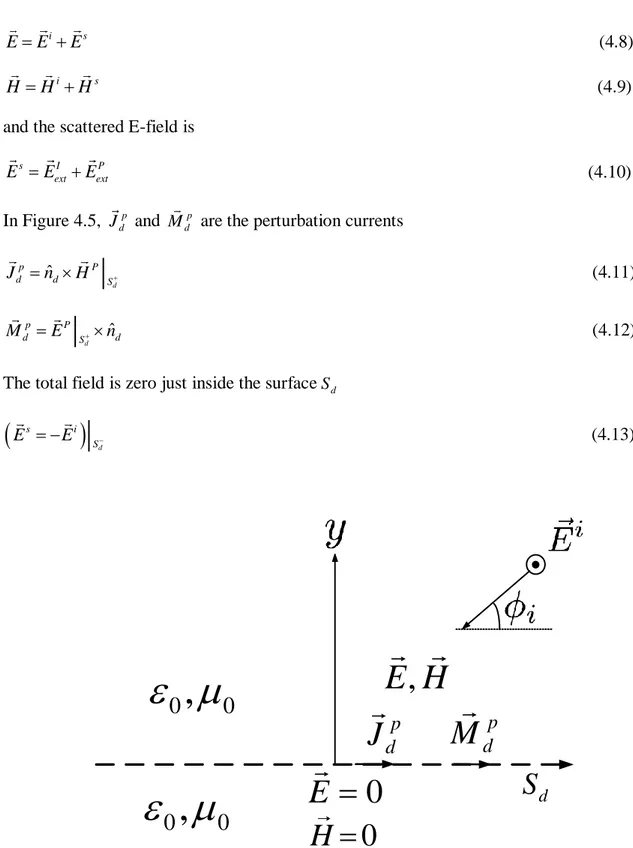
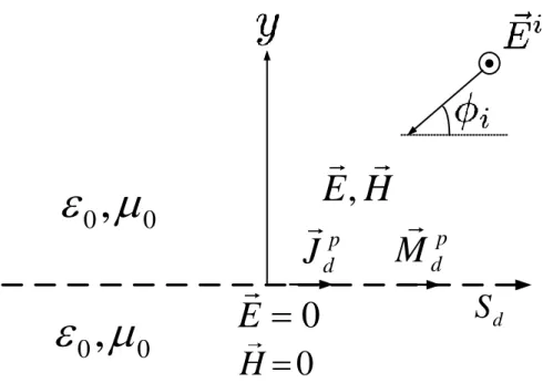
Figure 4. 1 The geometry of the problem... 31

Figure 4. 2 The flat surface as a scatterer ... 32

Figure 4. 3 External equivalence applied to the problem in Figure 4.2 ... 33

Figure 4. 4 Internal equivalence applied to the problem in Figure 4.2 ... 33

Figure 4. 5 The external equivalence principle applied to the problem in Figure 4.1 .. 34

Figure 4. 6 The internal equivalence principle applied to the problem in Figure 4.1 ... 35

Figure 4. 7 The geometry of the problem... 38

xi

Figure 4. 9 The internal equivalence principle applied to the problem in Figure 4.7 ... 40 Figure 4.10 The equivalence principle for the points inside of the cylinder applied to

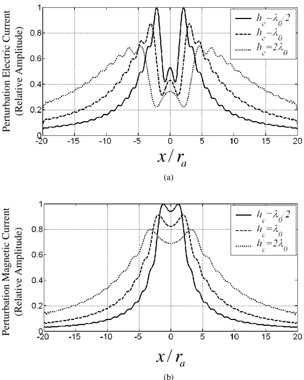
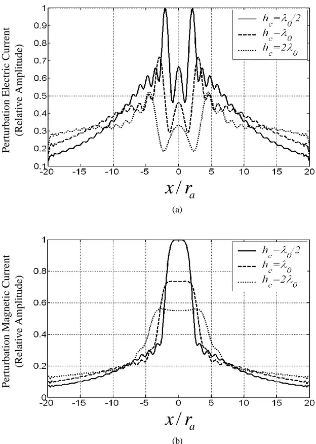
the problem in Figure 4.7 ... 41 Figure 4.11 The geometry used for the numerical results ... 43 Figure 4.12 Perturbation (a) electric currents normalized with 0.0016 A/m and (b)

magnetic currents normalized with 0.2968 V/m on the flat surface above the PEC object for f=1 GHz,  _i  _s 90, r_a ₀/ 3 m, x /r_{c a} 0.0,

1 15 0

   F/m, ₁₀ H/m and ₁ 0.0 Sm-1 ... 44 Figure 4.13 Perturbation (a) electric currents normalized with 0.00073 A/m and (b)

magnetic currents normalized with 0.16 V/m on the flat surface above the dielectric object for f=1 GHz, _i  _s 90, r_a ₀/ 3 m, x /r_{c a} 0.0,

1 15 0

   F/m, ₂ 4₀ F/m, ₁ ₂ ₀ H/m and ₁₂ 0.0 Sm-1 45 Figure 4.14 Perturbation (a) electric currents normalized with 0.0014 A/m and (b)

magnetic currents normalized with 0.2627 V/m on the flat surface above the PEC object for f=1 GHz,  _i  _s 90, r_a ₀/ 3 m, h_c ₀ m,

0.0

c a

x /r  , ₁15₀ F/m, and ₁₀ H/m ... 46 Figure 4.15 Perturbation (a) electric currents normalized with 0.00051 A/m and (b)

magnetic currents normalized with 0.12 V/m on the flat surface above the dielectric object for f=1 GHz,  _i  _s 90, r_a ₀/ 3 m, h_c ₀ m,

0.0

c a

x /r  , ₁15₀ F/m, ₂ 4₀ F/m, and ₁ ₂ ₀ H/m ... 47 Figure 4.16 Scattered field from the PEC object (a) normalized amplitude and (b) phase

for r_a 0.01m,  _i  _s 90, h /r_{c a} 1.0, x_c/r_a 0.0, wl /r_a 500, 1 0

  F/m, ₁0.0 Sm-1 and ₁₀ H/m ... 48 Figure 4.17 Scattered field from the dielectric object (a) normalized amplitude and (b)

phase for r_a 0.01m,  _i  _s 90, h /r_{c a} 1.0, x_c/r_a 0.0, wl /r_a 500 ,  ₁ ₀ F/m, ₂ 4₀ F/m, ₁₂ 0.0 Sm-1 and ₁₂ ₀ H/m . 49 Figure 4.18 The approximation difference of the method applied to the PEC object for

f=1 GHz,  _i  _s 90, r_a ₀ / 3 m, h_c/r_a 2.0, x / r_{c a} 0.0,  ₁ ₀ F/m, ₁0.0 Sm-1 and ₁₀ H/m ... 50 Figure 4.19 The approximation difference of the method applied to the dielectric object

for f=1 GHz,  _i  _s 90, r_a ₀/ 3 m, h_c/r_a 2.0, x / r_{c a} 0.0,  ₁ ₀ F/m, ₁4₀ F/m, ₁₂ 0.0 Sm-1 and ₁₂ ₀ H/m ... 51 Figure 4.20 A cylindrical object with elliptical cross-section ... 52 Figure 4.21 Relative scattered amplitude from a PEC cylindrical object with elliptical

cross-section for f=1 GHz, r_a 0.2 m, r_b 0.1 m, h / r_{c b} 1.0, 0.0

c a

x / r  , ₁15₀ F/m, ₁₀ H/m and ₁0.01 Sm-1 ... 52 Figure 4.22 Relative scattered amplitude from a PEC cylindrical object with elliptical

cross-section for f=1 GHz, _i 90, r_a 0.2 m, r_b 0.1 m, x / r_{c a} 0.0, 1 15 0

   F/m, ₁₀ H/m and ₁0.01 Sm-1 ... 52 Figure 4.23 Scattered amplitude from a dielectric cylindrical scatterer with circular

cross-section for r_a 0.01 m, h_c 0.01m, x_c/r_a 0.0, ò₁15ò F/m, ₀ 2

1 0

xii

Figure 5.1 Geometry of cylindrical object buried inside a lossy half-space with periodic surface ... 55 Figure 5.2 The geometry used for the numerical results ... 57 Figure 5.3 Perturbation (a) electric and (b) magnetic currents on the surface for f 1 GHz,  _i  _s 90, r_a ₀ 3 m, wl r_a 40, w_p 2₀ 3 m, h_p w_p 0.25, / 0.0 c a x r  , ₁ 15₀ F/m, ₂ 2.25₀ F/m, ₁ ₂ ₀ H/m, 1 0.001   Sm-1 and ₂ 0.0 Sm-1 ... 58 Figure 5.4 Scattered field (a) normalized amplitude and (b) phase for  _i  _s 90,

0.1 a r  m, w_p 0.2 m, h_p w_p 0.25, x_c/r_a 0.0, h_c/r_a 5.0, 50 a wl r   ₁ ₀ F/m, ₂ 4₀ F/m, ₁ ₂ ₀ H/m, and ₁ ₂ 0.0 Sm-1 ... 59 Figure 5.5 The approximation difference for f 1 GHz,  _i  _s 90, r_a ₀ 3 m,

0 2 3 p w   m, h_p w_p 0.25, x_c/r_a 1.0, h_c/ r_a 5.0,  ₁  ₀ F/m, 0 2 4    F/m, ₁₂ ₀ H/m, and ₁₂ 0.0 Sm-1 ... 60 Figure 5.6 Scattered amplitude from a cylindrical scatterer with circular cross-section for r_a 0.16₀ m, w_p 0.25₀m ... 61 Figure 5.7 Scattered amplitude from a cylindrical scatterer with circular cross-section

for r_a 0.16₀ m, w_p 0.4₀m ... 61 Figure 5.8 Scattered amplitude from a cylindrical scatterer with circular cross-section

for r_a 0.16₀ m, w_p 0.6₀m ... 62 Figure 5.9 Scattered amplitude from a cylindrical scatterer with circular cross-section

for r_a 0.16₀ m, w_p 2₀m ... 62 Figure 5.10 Scattered amplitude from a cylindrical scatterer with circular cross-section

for r_a 1.0₀ m, w_p 0.25₀m ... 63 Figure 5.11 Scattered amplitude from a cylindrical scatterer with circular cross-section

for r_a 1.0₀ m, w_p 0.4₀m ... 63 Figure 5.12 Scattered amplitude from a cylindrical scatterer with circular cross-section

for r_a 1.0₀ m, w_p 0.6₀m ... 64 Figure 5.13 Scattered amplitude from a cylindrical scatterer with circular cross-section

for r_a 1.0₀ m, w_p 2.0₀m ... 64 Figure 5.14 The approximation difference for f 400 MHz, _i 30, r_a 0.16₀ m,

0 0.6 p w   m, h_p 0.0064₀, x_c/r_a 0.0, h_c 0.17₀, wl h_c 10, 1 (4 0.01) 0 c j     F/m, ₂ 2.25₀ F/m, ₁ ₂ ₀ H/m, and ₂ 0.0 Sm-1 ... 65 Figure 5.15 Relative scattered amplitude from a cylindrical scatterer with circular cross-section for f 100 MHz, _i 20, w_p 2 /k₀ m, h_p 0.2 /k₀, wl h_c 10, F/m, ₁ 4₀ F/m, ₂ ò₀ F/m, ₁₂ ₀ H/m, ₁0.001 Sm-1 and

2 0.0

  Sm-1 ... 66 Figure 6.1 The incident E-field waveform a) in frequency domain b) in time domain . 68 Figure 6.2 TMz backscattered field from a cylindrical PEC object with r_a 0.01 m a) in frequency domain b) in time domain ... 70

xiii

Figure 6.3 TMz backscattered field from a buried cylindrical PEC object for ra 0.01

m, h_c 0.1m, x_c/r_a 0.0, ₁15₀ F/m, ₁₀ H/m,  _i  _s 90, and 1 0.001

  Sm-1 a) in frequency domain, b) in time domain ... 71 Figure 6.4 Expected reflections from a buried cylindrical object ... 72 Figure 6.5 TMz backscattered field from a buried cylindrical PEC object for r_a 0.01

m, h_c 0.01m, x_c/r_a 0.0, ₁ 15₀ F/m, ₁₀ H/m,  _i  _s 90, and ₁0.001 Sm-1 a) in frequency domain, b) in time domain ... 74 Figure 6.6 TMz backscattered field from a buried cylindrical PEC object for ra 0.01

m,h_c 0.1m, x_c/r_a 0.0, ₁ 15₀ F/m, ₁₀ H/m,  _i  _s 20, and 1 0.001

  Sm-1 a) in frequency domain, b) in time domain ... 75 Figure 6.7 TMz backscattered field from a buried cylindrical PEC object for r_a 0.01

m, h_c 0.1m, x_c/r_a 0.0, ₁15₀ F/m, ₁₀ H/m, and  _i  _s 90

a) in frequency domain (₁ 0.1 Sm-1), b) in time domain ... 76 Figure 6.8 TMz backscattered field from a cylindrical dielectric object for r_a 0.01 m,

1 4 0

   F/m, and ₁₀ H/m a) in frequency domain, b) in time domain ... 77 Figure 6.9 TMz backscattered field from a buried cylindrical dielectric object for

0.01

a

r  m,h_c 0.1m, x_c/r_a 0.0, ₁15₀ F/m, ₂ 4₀ F/m, 1 0.001

  Sm-1, ₂ 0.0 Sm-1, ₁₀ H/m, and  _i  _s 90 a) in frequency domain, b) in time domain ... 78 Figure 6.10 TMz backscattered field from a buried cylindrical PEC object for ra 0.01

m, h_c 0.1 m, x_c/r_a 0.0, ₁15₀ F/m, ₁₀ H/m,  _i  _s 90 ,

0.1

p

w  m, h_p/w_p 0.1 a) in frequency domain, b) in time domain ...79 Figure 6.11 TMz backscattered field from a buried cylindrical PEC object for ra 0.01

m, h_c 0.1 m, x_c/r_a 0.0, ₁15₀ F/m, ₁₀ H/m,  _i  _s 20 ,

0.1

p

w  m, h_p/w_p 0.1 a) in frequency domain, b) in time domain ... 80 Figure 6.12 TMz backscattered field from a buried cylindrical dielektrik object for

0.01 a r  m, h_c 0.1, x_c/r_a 0.0, ₁ 15₀ F/m, ₂ 4₀ F/m, 2 1 0    H/m,  _i  _s 20 , w_p 0.1, h_p /w_p 0.1 ... 80 Figure App. B.1 Evaluation of the self terms ... 87 Figure App. B.2 Evaluation of Principle Value ... 88

xiv

ABSTRACT

COMPUTATION OF ELECTROMAGNETIC FIELDS SCATTERED

BY CYLINDRICAL TARGETS BURIED IN A MEDIUM WITH A

PERIODIC SURFACE

Senem MAKAL

Department of Electronics and Communications Engineering Ph.D. Thesis

Advisor: Assoc. Prof. Dr. Ahmet KIZILAY

Electromagnetic scattering from a two dimensional, cylindrical, and dielectric object of arbitrary cross-section buried in a lossy dielectric half-space having a periodically rough surface is investigated by a new numerical method. The method is outlined for TMz (horizontally) polarized incident wave.

The basis of the new solution technique is that if a target is close to the surface, the electromagnetic fields will be nearly identical to that without the target, except within the region of finite extent near the target. Thus, the current on the surface will be affected only in a finite portion of the surface near the target. The electric field integral equations (EFIEs) for the equivalent currents on the target and the perturbation equivalent currents (the difference currents with target present and with target absent) on the surface are obtained by using this approach and solved by the Method of Moment (MoM) in frequency domain. Then, inverse Fourier transform is utilized to get the time domain signals. The short-pulse scattering results is used to investigate the effects of multipath.

Key Words: Electromagnetic scattering, the Method of Moment, perturbational field, integral equations.

YILDIZ TECHNICAL UNIVERSITY GRADUATE SCHOOL OF NATURAL AND APPLIED SCIENCE

xv

ÖZET

PERİYODİK BİR YÜZEY ALTINA GÖMÜLÜ SİLİNDİRİK

HEDEFLERDEN SAÇILAN ELEKTROMAGNETİK ALANLARIN

HESAPLANMASI

Senem MAKAL

Elektronik ve Haberleşme Mühendisliği Anabilim Dalı Doktora Tezi

Danışman: Doç. Dr. Ahmet KIZILAY

Sonsuz uzun, engebeli ve kayıplı bir dielektrik ortamda gömülü bir dielektrik hedeften saçılan elektromagnetik dalganın elektriksel alan değeri TMz polarizasyonu için perturbasyon yaklaşımı ile çözülmüştür.

Kullanılan bu yeni çözüm metodunun temeli, eğer hedef cisim periyodik yüzeye yakın ise, elektromanyetik alanların hedef cismin bulunmadığı durumdaki alanlar ile sadece hedef cisme yakın sonlu bir bölgede farklı olacağına ve bu sayede periyodik yüzeydeki eşdeğerlik akımının hedef cismin hemen üzerindeki sonlu bir yüzeyde değişiklik göstereceğine dayanmaktadır. Bu yaklaşımla silindirik hedefin üzerindeki eşdeğerlik akımlarına ve sinüzoidal yüzey üzerindeki perturbasyon (hedefin olduğu ve olmadığı durumlardaki eşdeğer akımlar arasındaki fark akımı) eşdeğerlik akımlarına ait elde edilen elektrik alan entegral denklemleri, frekans domeninde Moment Metodu kullanarak çözülmüş ve bu sayede geniş bantta, saçılan elektrik alana ait çözümler elde edilmiştir. Sonrasında, ters Fourier dönüşümü ile zaman domeni işaretleri bulunmuş ve böylece kısa darbe saçılma işaretleri kullanılarak çoklu yansıma etkileri incelenmiştir. Anahtar Kelimeler: Elektromagnetik alanlar, Moment Metodu, perturbasyon alanları, integral denklemleri.

1

CHAPTER 1

INTRODUCTION

1.1 Literature

Solution of the electromagnetic scattering by buried objects has been interested by many researches. Therefore, several techniques have been employed to obtain the scattered fields. This is because scattered field values can be used in nondestructive evaluation applications such as detecting landmines, buried pipes, near-surface geophysical exploration, and also archeological studies [1-7]. As a result, an efficient way of calculating scattered field is important for ground-penetrating radar applications.

Many different techniques have been developed for two-dimensional scattering from buried objects. Especially, a large number of exact and numerical techniques are related to the assumption of a flat interface, because of the reduction of mathematical and computational complexity. For example, Uzunoglu et al. have computed the scattered electric field from underground tunnels using a Green's function approach, and analyzed the scattered amplitude for various observation angles [8]. Kanellopoulos et al. have used the same analytical approach for conducting wires buried in earth [9]. Also, Born approximation and Sommerfield integrals with fast evaluation methods have been the other ways to build an analytical solution for buried scatterer [10-12]. Naqvi et al. have used plane wave expansion and excitation of current on a cylinder for the scattered electric field from a conducting cylinder deeply buried in a dielectric half-space [13]. Another analytical method containing plane wave representation has been developed by Ahmed et al. [14].

2

In case the surface of the half-space is rough, Cottis and Kanellopoulos assume a sinusoidal interface and use an integral equation combined with the extended boundary condition approach for the scattering from a buried circular cylinder in [15] and [16]. An analytical solution of the scattering problem from a dielectric cylinder buried beneath a slightly rough surface is developed by Lawrence and Sarabandi [17]. Altuncu et al. present a method using the Green’s function of the half-space with rough boundary where the cylindrical bodies are located [18].

1.2 The Aim of the Thesis

The aim of this thesis is to obtain a fast and simple solution method for the complex problem of calculation of the scattered fields from a cylindrical object buried under a rough surface. This new solution technique is outlined for TMz scattering from a cylindrical object buried in a lossy half-space. The surface equivalence principle and a perturbation method are employed to form a set of EFIEs for the currents on the object and the portion of the surface most strongly interacting with the object. Then, MoM is used to solve the EFIEs in the frequency domain to obtain the scattered electric field, and inverse Fourier transform is utilized to get the time domain signals.

1.3 Hypothesis

The idea behind the new solution technique is that if a target is close to the surface, the electromagnetic fields will be nearly identical to that without the target, except within the region of finite extent near the target [19, 20]. Thus, the current on the surface will be affected only in a finite portion of the surface near the target. Therefore, the perturbation equivalent currents are approximated to zero outside a finite region above the object. The EFIEs are solved in the frequency domain using MoM, and transformed into the time domain using IFT.

3

CHAPTER 2

COMPUTATION OF TM

z

SCATTERING FROM A CYLINDRICAL

DIELECTRIC OBJECT

2.1 Introduction

The problem of electromagnetic scattering from a two-dimensional, dielectric, and cylindrical object of arbitrary cross section is considered. First, the analytical solution of the problem is obtained. Then, the surface equivalence principle is used for the numerical solution of the same problem. Numerical solution method is outlined for the case of arbitrary cross-section, and specialized for circular cross-section. Finally, computed results of these two solutions are compared.

2.2 Analytical Solution

The scattered electric field from a dielectric cylindrical object of circular cross section is calculated by expressing the plane waves by cylindrical wave functions [21, 22]. As shown in Figure 2.1, TMz polarized incident wave

 

Ei _{is assumed to be incident with} the incidence angle of _i on the object having a radius r . The surface of the object is _a

represented by S . _c

The plane waves can be represented by an infinite sum of cylindrical wave functions, and the incident electric field [21, 22]

 

0 0 ˆ ˆ i i n jn z n n E zE zE j J k  e      



(2.1)

4

c

S

0

,

0

 

a

r

1

,

1

,

1

  

Figure 2. 1 An infinitely long cylindrical object of circular cross-section.

since it must be periodic in  and finite at  0, where  is the magnitude of the two-dimensional position vector. Here, k₀ is the free-space wave number. The position vector

ˆ ˆ

xx yy

   (2.2) The scattered electric field in the region exterior to the cylinder

 2

_{ }

0 0 ˆ s n jn n n n E zE j a H k  e     



(2.3) and the total field in the cylinder

 

0 1 ˆ t n jn n n n E zE j b J k e     



(2.4) where k₁   _{1 c1} , and _{1 1} 1 1 1 c j        _  _

 . The magnetic field can be computed

from the electric field (E-field), and therefore [21, 22]

 

0 0 0 0 1 _ˆ i i n jn n n E H E j J k e j j             



(2.5)

5  2

_{ }

0 0 0 0 1 _ˆ s s n jn n n n E H E j a H k e j j             



(2.6)

 

0 1 1 1 1 _ˆ t t n jn n n n E H E j b J k e j j             



(2.7) where ₀   ₀ / ₀ and ₁   ₁/ _c1 are the intrinsic impedance of free half-space and lossy dielectric, respectively. The unknown coefficients a and _n b can be found by _n

applying the boundary condition of



,





,





,



i s t z a z a z a E r  E r  E r  (2.8)



,





,





,



i s t a a a H_ r



H_ r



H_ r



(2.9) More explicitly, for the tangential electric and magnetic field on the boundary [21,22]





 2

_

_

_{ }

0 0 0 0 0 1 n jn n jn n jn n a n n a n n a n n n E j J k r e  E j a H k r e  E j b J k r e            







(2.10)





 

_

_

 

2 0 0 0 0 0 0 0 1 1 n jn n jn n a n n a n n n jn n n a n E E j J k r e j a H k r e j j E j b J k r e j                    







(2.11)

Taking advantage of the orthogonality of Bessel functions





 2

_

_

_{ }

0 0 0 0 0 1 n n n n a n n a n n a E j J k r E j a H k r E j b J k r (2.12)





 2

_

_

_{ }

0 0 0 0 0 1 0 0 1 n n n n a n n a n n a E E E j J k r j a H k r j b J k r     _{ }  _{ }  _{ (2.13)}

Solving the equations (2.12) and (2.13), the unknown coefficients a and _n b _n

   

   

 

 

_{ }

_{ }

 

_{ }

1 0 1 0 0 1 2 2 0 1 0 1 1 0 n a n a n a n a n n a n a n a n a J k r J k r J k r J k r a J k r H k r J k r H k r            (2.14)





 

_

_

_

_

 

_

_

 

 

_

_

_{ }

 

_

_

2 2 0 0 0 0 1 2 2 0 1 0 1 1 0 n a n a n a n a n n a n a n a n a J k r H k r J k r H k r b J k r H k r J k r H k r           (2.15)

The scattered E-field is calculated by using a coefficient. Large argument _n

6

 

0 0 (2) 0 0 0 2 lim jk k j e H k k         (2.16)

Thus, the scattered E-field in the far zone



      n jn n n jk s e a j e k j E z E     0 0 0 2 ˆ  (2.17) 2.3 Numerical Solution

Although there are exact solutions for scattering by cylinders of circular and elliptical cross-section, calculation of scattered fields from cylinders of arbitrary cross-section are obtained by numerical methods [23-25]. Here, to analyze the accuracy of the numerical solution, the surface equivalence principle and MoM are used for the same problem.

2.3.1 The Surface Equivalence Principle

In the surface equivalence principle, actual sources such as an antenna are replaced by equivalent sources [21-25]. The fields outside an imaginary closed surface are obtained by replacing the electric and magnetic equivalent currents radiating in unbounded media and satisfying the boundary conditions. If the currents are selected so that the fields inside the closed surface are zero or any other value and the field at an arbitrary point outside is determined, this is called external equivalence. In external equivalence principle, the whole space parameters are chosen as the parameters of the exterior medium. If the currents are selected so that the fields outside the closed surface are zero or any other value and the field at an arbitrary point inside is determined, this is called internal equivalence. In internal equivalence principle, the whole space parameters are chosen as the parameters of the interior medium [25].

2.3.1.1 Theory

The surface equivalence principle is used to solve the scattered E-field by a two-dimensional cylindrical object of arbitrary cross section as shown in Figure 2.2.

7

0

0

,





c

S

c

nˆ

1

1

1

,



,





Figure 2. 2 An infinitely long cylindrical object of arbitrary cross-section.

In Figure 2.2, ˆn is the outward unit normal vector to _c S . The incident field is a TM_c z plane wave with angle _i from the horizontal

 

0 cos sin  0 ˆ , jk x i y i i E x y z E e   (2.18) Figure 2.3 shows the external equivalence principle applied to the problem in Figure 2.2. The whole space parameters are chosen as



 ₀, ₀



[26, 27]. The surface is replaced by surface electric (Jc) and magnetic (Mc) currents

ˆ c c c _S J  n H  (2.19) ˆ c c S c M E n (2.20) At any point outside the surface, the total fields are E and H . The total fields are zero under the surface



,



 

c c

s i

ext c c _{S S}

8

0

0

,





c

S

c

J



,

E H

0

0





H

E





0

0

,





c

M



Figure 2. 3 The external equivalence principle applied to the problem in Figure 2.2. Here, ext means external and S_c represents the surface just inside S_c. Then, the internal equivalence principle is applied in Figure 2.4 to the problem shown in Figure 2.2. Therefore, the whole space parameters are chosen as



  ₁, ₁, ₁



[26, 27]. The surface is replaced by (Jc) and (Mc). The total fields are zero at any point external toSc



,



0

c

s

int c c S

E



J



M





(2.22)

Here, int means internal, and S_crepresents the surface just outside S_c.

In other words, there are two equations (2.21) and (2.22) to be solved by using MoM and two unknown currents to calculate the scattered field. The E-field is expressed in terms of electric and magnetic potential functions [23], and equations (2.21) and (2.22) can be rewritten as

 

 

0 1 , ext e i c c z xt z z c j A J F M E S       _ _   (2.23)

 





1 1 0, int int c c c c z z j A J F M S        _  _  (2.24)

9

c

S

,

E H

0

0





H

E





c

J





c

M



1

1

1

,



,





1

1

1

,



,





Figure 2. 4 The internal equivalence principle applied to the problem in Figure 2.2. where A and F denote the magnetic and electric vector potential, respectively. They are given by the following line integrals

 

 

(2)





0 4 j C A J H k dl j          



(2.25)

 

 

(2)





0 4 m C F M H k dl j          



(2.26) where  

is a two-dimensional position vector for source points

ˆ ˆ

x x y y

    (2.27) The contours over J _{and M are} C_j and C , respectively. The two equations (2.23) _m

and (2.24) are solved numerically using MoM for two unknown surface currents (Jc,Mc).

2.3.1.2 MoM Solution

The currents on the surfaces of S_d and S are approximated by linear segments as _c

shown in Figure 2.5.

 

 

1 ˆ c N c c c i i i J  z I P       



(2.28)

10

 

 

1 ˆ c c N i i i c c i M   K P       



(2.29) where N_c is the number of segments on S . _c c

i

I and c i

K are the unknown values of electric and magnetic current on the i th segment of S , respectively. The unit vector in _c

the circumferential direction tangent to the ith segment of S is denoted by ˆ_c _i, and the unit vector in the z-direction is denoted by ˆz. Pulse functions (Pc) are chosen as the expansion functions and defined as unity on segment Cci.

Segment C

ci i i+1 i+2 i+3 n



n+1 n+2 n+3

Figure 2. 5 Linear segmentation of the cylindrical object.

Using equation (2.26) and (2.29), it is explained in detail in Appendix A and can be shown that

 

)









1 0 (2 0 1 0 ˆ 4 1 c ci c N i c x i e t c i _C n jk K k d F M H    l               

 

(2.30)

Equations (2.23) and (2.24) can be rewritten using point matching at N_c points on the surface, the coupled EFIEs become

11













(2) 0 0 0 1 (2) 0 1 0 1 4 ˆ , 4 c ci c ci N c i i C c N i c i i z c i C I H k dl n jk K H k dl E S  _{ }                        

 

 

(2.31)













(2) 1 0 1 1 (2) 1 1 1 1 4 ˆ 0 , 4 c ci c ci N c i i C c N i c i c i _C I H k dl n jk K H k dl S  _{ }                      

 

 

(2.32) where (2) 0

H is the zeroth-order Hankel function of the second kind, and (2) 1

H is the first-order Hankel function of the second kind. After pulse weighting functions are used to transform these EFIEs to linear equations, they can be written in matrix form

1 1 2 2 0 c C M c c C M Z Z I V Z Z K     _              (2.33)

Here, Z , _C1 Z_C2, Z_M1, and Z_M2 are the square sub matrixes of N_cN_c. The element in the ith row and the nth column of these matrixes is equal to the E-field at the midpoint of the nth segment of S , produced by electric and magnetic currents lying on the ith _c

segment of S . The left hand side of the equation is the column sub vectors containing _c

the unknown expansion coefficients. The right hand side of the equation contains the incident field on S . The ith element of _c V is the incident field at the middle of the ith _c

segment of S . _c

The self terms



  



should be calculated carefully, because the argument of the Hankel functions becomes very small and the integration of the Hankel function becomes difficult to compute numerically. Therefore, the self-terms should be approximated by using the Hankel function terms for small arguments [28] as shown in Appendix B.





(2) 0 2 1 ln 1 4 ci C c k c H k   dl j            _  _{  } _        



(2.34)









(2) 1 ˆ 2 ci c i C n j H k dl k               



(2.35)

12

where c is the length of the segment on S and _c  1.781.

The unknown expansion coefficients are solved and the far scattered field can be computed by using J_c and M_c

    0 0 0 0 cos sin 0 1 0 cos sin 0 1 0 2 4 2 4 c s s c s s c c N jk jk x y s z i i i N jk jk x y i i c c i j e E I e k jk j e K e k                            





(2.36)

where _s is the scattering angle.

2.4 Numerical Results

In the two-dimensional case, the scattering radar cross section is given by [29]

 





2 , lim 2 s z s s i z E E         (2.37)

Figure 2.6 shows the scattering cross section of a circular dielectric cylinder calculated by both analytical and numerical methods. There are three different numerical results obtained by changing the points per free-space wavelength ( ppw ) used to represent the currents on the object. In figures, free-space wavelength is indicated by (₀). As it is seen that the ppw increases, there is an excellent agreement between the analytical and numerical solutions.

13 0



a

r

0

2





TM

Figure 2. 6 Scattering cross section of a circular dielectric cylinder for f 1GHz,

20

s i

 _{ } 

14

CHAPTER 3

COMPUTATION OF TM

z

SCATTERING FROM A CYLINDRICAL

OBJECT COATED WITH A DIELECTRIC MATERIAL

3.1 Introduction

In this chapter, the problem of electromagnetic scattering from a two-dimensional cylinder of arbitrary cross section coated with a dielectric material is considered. First, the analytical and numerical solutions of the problem relating to the conducting cylindrical object coated with a dielectric material are given, and then computed results of these two solutions are compared for the case of circular cross-section. Then, these steps are also applied for the problem relating to the dielectric cylindrical object coated with a dielectric material.

3.2 Scattering from a Conducting Cylindrical Object Coated with a Dielectric Material

3.2.1 Analytical Solution

The scattered E-field from a conducting cylindrical object coated with a dielectric material is calculated by expressing the plane waves by cylindrical wave functions. As shown in Figure 3.1, conducting and dielectric objects have circular cross-section. The radius and the surface of the coated cylinder are r and _b S ; respectively. _d

15

c

S

0 0

,





1

, ,

1 1

  

a

r

b

r

d

S





2



Figure 3. 1 A conducting cylindrical object of circular cross-section coated with a dielectric cylindrical object of circular cross-section

As mentioned in chapter 2, the incident E-field [21, 22]

 

0 0 ˆ ˆ i i n jn z n n E zE zE j J k  e      



(3.1) The scattered E-field in the region exterior to the dielectric cylinder

 2

_{ }

0 0 ˆ s n jn n n n E zE j a H k  e     



(3.2) and the total field in the dielectric cylinder

 

 

0 1 0 1 ˆ ˆ t n jn n jn n n n n n n E zE j b J k  e  zE j c Y k e        







(3.3)

The magnetic field can be computed from the E-field, and therefore [21, 22]

 

0 0 0 0 1 _ˆ i i n jn n n E H E j J k e j j             



(3.4)  2

_{ }

0 0 0 0 1 _ˆ s s n jn n n n E H E j a H k e j j             



(3.5)

 

 

0 0 1 1 1 1 1 1 _{ˆ ˆ} t t n jn n jn n n n n n n E E H E j b J k e j b Y k e j j j                     







(3.6)

16

The unknown coefficients a , _n b and _n c_n can be found by applying the boundary condition of



,





,





,



i s t z b z b z b E r  E r  E r  (3.7)



,





,





,



i s t b b b H_ r



H_ r



H_ r



(3.8)



,



0 t a E r   (3.9) More explicitly, for the tangential electric and magnetic field on the boundary [21, 22]





 

_

_

_{ }

 

2 0 0 0 0 0 1 0 1 n jn n jn n jn n b n n b n n b n n n n jn n n b n E j J k r e E j a H k r e E j b J k r e E j c Y k r e                   









(3.10)

 

 

_{ }

 

 

2 0 0 0 0 0 0 0 0 1 1 1 1 n jn n jn n b n n b n n n jn n jn n n b n n b n n E E j J k r e j a H k r e j j E E j b J k r e j b Y k r e j j                           









(3.11)

 

 

0 1 0 1 0 n jn n jn n n a n n a n n E j b J k r e  E j c Y k r e         





(3.12)

Taking advantage of the orthogonality of Bessel functions





 2

_

_

_{ }

_{ }

0 0 0 0 0 1 0 1 n n n n n b n n b n n b n n b E j J k r E j a H k r E j b J k r E j c Y k r (3.13)





 2

_

_

_{ }

_{ }

0 0 0 0 0 0 1 1 0 0 1 1 n n n n n b n n b n n b n n b E E E E j J k r j a H k r j b J k r j c Y k r      _{ }  _{ }  _{ }  _ (3.14)

 

 

0 1 0 1 0 n n n n a n n a E j b J k r E j c Y k r  (3.15)

Solving the equations (3.13), (3.14) and (3.15), the unknown coefficients a ,_n b_n and c_n

are calculated and the scattered E-field is calculated by using a coefficient [21, 22] _n

0 0 0 2 ˆ jk s n jn n n j e E zE j a e k         



(3.16)

17 3.2.2 Numerical Solution

To analyze the accuracy of numerical solution of this problem, the surface equivalence principle and MoM are used.

3.2.2.1 Theory

The surface equivalence principle is used to find the total field at an external point of the problem shown in Figure 3.2. It has two steps containing two equivalent and simpler problems. Figure 3.3 shows the external equivalence problem. The whole space parameters are chosen as



 ₀, ₀



. The surface is replaced the equivalent surface electric current by J_d and the equivalent surface magnetic current M_d[26, 27]

ˆ d d d S J n H  (3.17) ˆ d d _S d M E n (3.18) where ˆn_d is the outward unit normal vector to S . _d

0 0

,





c

S

c

nˆ

1 1 1

,



,









2



d

S

d

nˆ

Figure 3. 2 An infinitely long conducting cylindrical object of arbitrary cross-section coated with a dielectric cylindrical object of arbitrary cross-section

18

At any point outside the surface, the total fields are E and H . The total field is zero

inside S denoted _d S_d



,



 

d d s i ext d d S S E J M   E  (3.19)

Figure 3.4 shows the internal equivalence problem. The whole space parameters are chosen as



  ₁, ₁, ₁



. The total field is zero on both S_d and S_c



, ,



0 d s int d d c S E J M J   (3.20)



, ,



0 c s int d d c S E J M J   (3.21) 0 0

,





d

S

0 0

,





,

E H

0

0





H

E





d

J



d

M



Figure 3. 3 The external equivalence principle applied to the problem in Figure 3.2. where S_drepresents the surface just outside S_d.

19 c

S

1 1 1

,



,





d

S

1 1 1

,



,





,

E H

0

0





H

E





0

0





H

E





d

J





d

M





c

J



Figure 3. 4 The internal equivalence principle applied to the problem in Figure 3.2. In other words, there are three equations (3.19), (3.20) and (3.21) to be solved by using MoM and three unknown currents to calculate the scattered field. The E-field is expressed in terms of electric and magnetic potential functions, and equations (3.19), (3.20) and (3.21) can be rewritten as [26, 27]

 

 

0 1 , ext e i d d z xt z z d j A J F M E S       _ _   (3.22)

 





 

1 1 , 0 z z

int int int

d d c d c z j A J F M j A J S        _  _   (3.23)

 





 

1 1 , 0 z z

int int int

d d c c c z j A J F M j A J S        _  _   (3.24)

Three equations (3.22)-(3.24) are solved numerically using MoM for three unknown surface currents (J_d,M_d,J_c).

3.2.3 MoM Solution

The currents on the surfaces of S_d and S_c are approximated by linear segments [26, 27]

 

 

1 ˆ d N i i i d d d J  z I P       



(3.25)

20

 

 

1 ˆ d d N i i i d d i M   K P       



(3.26)

 

 

1 ˆ c N i i i c c c J  z I P       



(3.27) where N_d is the number of segments on S . _d d

i

I and d i

K are the unknown values of electric and magnetic current on the i th segment of S , respectively. _d

Equations (3.22)-(3.24) can be rewritten using equations (3.25)-(3.27)













(2) 0 0 0 1 (2) 0 1 0 1 4 ˆ , 4 d di d di N d i i C d N i d i i z d i _C I H k dl n jk K H k dl E S  _{ }                        

 

 

(3.28)

















(2) 1 0 1 1 (2) 1 1 1 1 (2) 1 0 1 1 4 ˆ 4 0 , 4 d di d di c ci N d i i C d N i d i i C N c i d i C I H k dl n jk K H k dl I H k dl S  _{ }        _{ }                     

 

 

 

(3.29)

















(2) 1 0 1 1 (2) 1 1 1 1 (2) 1 0 1 1 4 ˆ 4 0 , 4 d di d di c ci N d i i C d N i d i i C N c i c i C I H k dl n jk K H k dl I H k dl S  _{ }        _{ }                     

 

 

 

(3.30)

where C_d is the contour representing of S . _d

The unknown expansion coefficients are solved and the far scattered field can be computed using Jd and Md

21     0 0 0 0 cos sin 0 1 0 cos sin 0 1 0 2 4 2 4 d s d s s s N jk jk x y s d z i i i N jk jk x y d i i i d d j e E I e k jk j e K e k                            





(3.31)

where d is the length of the segment on S . _d

3.3 Scattering from a Dielectric Cylindrical Object Coated with a Dielectric Material

3.3.1 Analytical Solution

As shown in Figure 3.5, both of the dielectric objects have circular cross-section. The incident fields, the scattered fields in the region exterior to the cylinder having radius

b

r , and the total fields in the cylinder having radius r are calculated by expressing the _b

plane waves by cylindrical wave functions as shown in equations (3.1)-(3.6).

2 2 2

,



,





c

S

0

0

,





1

, ,

1

1

  

a

r

b

r

d

S

Figure 3. 5 A dielectric cylindrical object of circular cross-section coated with a dielectric cylindrical object of circular cross-section