REPUBLIC OF TURKEY
YILDIZ TECHNICAL UNIVERSITY
GRADUATE SCHOOL OF NATURAL AND APPLIED SCIENCES
ROBUST MOVING HORIZON
CONTROL OF DISCRETE
TIME STATE-DELAYED SYSTEMS
FATMA YILDIZ TAŞCIKARAOĞLU
PhD. THESIS
DEPARTMENT OF ELECTRICAL ENGINEERING
PROGRAM OF CONTROL AND AUTOMATION
ADVISER
REPUBLIC OF TURKEY
YILDIZ TECHNICAL UNIVERSITY
GRADUATE SCHOOL OF NATURAL AND APPLIED SCIENCES
ROBUST MOVING HORIZON
CONTROL OF DISCRETE
TIME STATE-DELAYED SYSTEMS
A thesis submitted by Fatma YILDIZ TAŞCIKARAOĞLU in partial fulfillment of the requirements for the degree of DOCTOR OF PHILOSOPHY is approved by the committee on 21.06.2013 in Department of Electrical Engineering, Control and Automation Program.
Thesis Adviser
Assoc. Prof. Dr. İbrahim Beklan KÜÇÜKDEMİRAL Yıldız Technical University
Co- Adviser
Assist. Prof. Dr. Şeref Naci ENGİN
Yıldız Technical University – Technology Transfer Office
Approved By the Examining Committee
Assoc. Prof. Dr. İbrahim Beklan KÜÇÜKDEMİRAL
Yıldız Technical University _____________________
Assoc. Prof. Dr. Haluk GÖRGÜN, Member
Yıldız Technical University _____________________
Prof. Dr. Leyla Gören SÜMER, Member
Istanbul Technical University _____________________
Prof. Dr. Galip CANSEVER, Member
Yıldız Technical University _____________________
Assoc. Prof. Dr. Erkan ZERGEROĞLU, Member
ACKNOWLEDGEMENTS
Above all, I would like to express the deepest gratitude to my advisor, Assoc. Prof. İbrahim Beklan Küçükdemiral for his expertise and valuable guidance throughout my Ph.D thesis. In addition, I am grateful to my co-adviser Dr. Şeref Naci Engin for his professional advices.
Also, I wish to deeply thank to my committee members, Prof. Dr. Leyla Gören Sümer and Assoc. Prof. Haluk Görgün for their invaluable comments and constructive feedbacks.
I also take this opportunity to express my special gratitude to Prof. Imura, who has initiated me into this field of study during my work in the Imura Laboratuary there. I am also thankful to my colleague, Dr. Levent Ucun, who provided assistance in the development and preparation of this thesis.
I am indebted to my parents for helping and supporting me all the time and I appreciate my husband, Akın Taşcıkaraoğlu for his encouragement and understanding.
Finally, I owe my loving thanks to my son, Selim who was born in the middle of my studies but has given me so much life energy and support for being so understanding for his small age.
June, 2013
TABLE OF CONTENTS Page
TABLE OF CONTENTS ... iv
LIST OF SYMBOLS ... vi
LIST OF ABBREVIATIONS ... vii
LIST OF FIGURES ... viii
LIST OF TABLES ... ix ABSTRACT ... x ÖZET ... xii CHAPTER 1 INTRODUCTION ... 1 1.1 Literature Review ... 1 1.2 Purpose of Thesis ... 5 CHAPTER 2 PRELIMINARIES ... 7 CHAPTER 3 TIME-DELAY SYSTEMS ... 11 3.1 System Description ... 11
3.2 Stability of Time-Delay Systems ... 12
3.2.1 Lyapunov-Razumikhin Theorem ... 12
3.2.2 Lyapunov-Krasovskii Theorem ... 13
3.2.4 Delay-Dependent Stability ... 14
CHAPTER 4 MOVING HORIZON CONTROL ... 16
4.1 Problem Formulation ... 16
4.2 Overview of Moving-Horizon Control... 17
4.2.1 Stability of the Moving-Horizon Control ... 18
4.2.2 Dissipativity of Moving-Horizon Control ... 19
CHAPTER 5 MOVING-HORIZON CONTROL FOR TIME-DELAY SYSTEMS ... 22
5.1 Problem Formulation ... 22
5.2 Stability of Delay Dependent Moving-Horizon Control ... 24
5.3 Robust Moving-Horizon Control For Time Delay Systems ... 27
5.3.1 Robust Stability Condition ... 27
5.3.2 Input Constraint ... 28 5.3.3 State Constraint ... 29 5.3.4 Dissipativity Condition ... 31 CHAPTER 6 NUMERICAL EXAMPLES... 37 CHAPTER 7 CONCLUSIONS ... 53 REFERENCES ... 55 CURRICULUM VITAE ... 59
LIST OF SYMBOLS
State feedback gain Lyapunov function Delay coefficient
Upper bound of time-delay Lower bound of time-delay Diagonal
Dissipation level
Delay based dissipation level Set of real numbers
Control input State-vector Disturbance input Measured output
Exogenous controlled output Disturbance bound coefficient
Performance index from disturbance to performance output
Performance index from disturbance to performance output without constraints Vector 2-norm
LIST OF ABBREVIATIONS
L-K Lyapunov-Krasovskii LMI Linear Matrix Inequality LPV Linear Parameter Varying MHC Moving Horizon Control MHHC Moving Horizon Control MPC Model Predictive Control RHC Receding Horizon Control RHHC Receding Horizon H∞ Control
BRL Bounded Real Lemma TDS Time Delay System
LIST OF FIGURES Page Figure 6.1 Linear state-space model (linmod) of the system with reference ... 37 Figure 6.2 The flowchart of the algorithm for the moving horizon control .... 39 Figure 6.3 PID control of the anaerobic system (a) Disturbance , (b) bacteria
growth curves in the reactors, , and substrate levels , (c)control input, (d) methane gas output . ... 40 Figure 6.4 Moving horizon control (− −) vs. control (─) on ... 41 Figure 6.5 Disturbance signal applied to the system ... 42 Figure 6.6 The variation of disturbance attenuation level, , for different delay
sizes. ... 43 Figure 6.7 The time-history of the controlled output, , and control input, , for
. ... 44 Figure 6.8 The time-history of the controlled output, , and control input, , for
. ... 45 Figure 6.9 The time-history of the controlled output, , and control input, , for
. ... 46 Figure 6.10 The time-history of the controlled output, and control input, for
. ... 47 Figure 6.11 The variations of disturbance attenuation level, , for different delay
intervals. ... 49 Figure 6.12 The time-history of the controlled output, , and control input, , for
. ... 50 Figure 6.13 The time-history of the controlled output, , and control input, , for
. ... 51 Figure 6.14 The time-history of the controlled output, , and control input, , for
. ... 52
LIST OF TABLES Page
Table 6.1 The parameters of the anaerobic system ... 38
Table 6.2 The PID coefficients computed by means of Ziegler-Nichols method. ... 40
Table 6.3 values at each step in Example 2 ... 43
ABSTRACT
ROBUST MOVING HORIZON CONTROL OF DISCRETE
TIME STATE-DELAYED SYSTEMS
Fatma YILDIZ TAŞCIKARAOĞLU
Department of Electrical Engineering Ph.D Thesis
Adviser: Assoc. Prof. Dr. İbrahim Beklan KÜÇÜKDEMİRAL Co-adviser: Dr. Şeref Naci ENGİN
This thesis is concerned with design of a delay-dependent type moving horizon state-feedback control (MHHC) for a class of linear discrete-time system subject to time-varying state delays, norm bounded uncertainties and disturbances with bounded energies. The closed-loop robust stability and robust performance problems are considered to overcome the instability and poor disturbance rejection performance due to the existence of parametric uncertainties and time-delay appeared in the system dynamics. The main objective is the development of possible low conservative stability condition for time-delay systems and of a novel control method for such systems using dissipation constraint together with on-line adapting of the dissipation level. For that purpose, the constrained minimax optimization problem is dealt with in the framework of Linear Matrix Inequality (LMI), in which the maximization is realized over a set of uncertainties and bounded disturbances. Utilizing a discrete-time Lyapunov-Krasovskii (L-K) functional, some delay-dependent, LMI based conditions are provided. It is shown that if one can find a feasible solution set for these LMI conditions iteratively in each step of run-time, then we can construct a control law which guarantees the closed-loop asymptotic stability, maximum disturbance rejection performance and closed-closed-loop dissipativity in view of the actuator limitations. Two numerical examples and simulations on a nominal and uncertain discrete-time, time-delayed systems, are presented at the end, in order to demonstrate the efficiency of the proposed method.
Key words: Moving horizon control, control, model predictive control, time-delay system, delay-dependent control, time-varying delay, robust stability.
ÖZET
DAYANIKLI MODEL ÖNGÖRÜLÜ KONTROL İLE
AYRIK ZAMANLI DURUM GECİKMELİ SİSTEMLERİN KONTROLÜ
Fatma YILDIZ TAŞCIKARAOĞLU
Elektrik Mühendisliği Anabilim Dalı Doktora Tezi
Tez Danışmanı: Doç. Dr. İbrahim Beklan KÜÇÜKDEMİRAL Eş Danışman: Dr. Şeref Naci ENGİN
Bu tez çalışmasında, zamanla değişebilen durum gecikmesi, normu sınırlandırılmış belirsizlikler ve sınırlı enerjiye sahip bozucu etkiler içeren doğrusal ayrık zamanlı sistemler için zaman gecikmesine bağlı geri-beslemeli model öngörülü kontrol yöntemi (MHHC) tasarımı üzerinde durulmuştur. Sistem dinamiklerinde bulunan belirsizliklerden ve zaman gecikmesinden kaynaklanan kararsızlığı ve kötü performansı önlemek amacıyla kapalı çevrim dayanıklı kararlılık ve dayanıklı performans problemleri ele alınmıştır. Çalışmanın temel hedefi, zaman gecikmeli sistemler için tutuculuğu düşük kararlılık şartı ve bu sistemler için çevrim içi değişen kayıplılık seviyesi ile kayıplılık kısıtını kullanarak yeni bir kontrol yöntemi geliştirmektir. Bu amaçla, en kötü durumun bir takım belirsizlikler ve sınırlı bozucu dahilinde bulunduğu kısıtlı minimax optimizasyon problemi Lineer Matris Eşitsizlikleri (LME) çerçevesinde ele alınmıştır. Kapalı çevrim sistemin asimptotik kararlılığını, performansını ve yitirgenliğini sağlamak amacıyla ayrık zamanlı Lyapunov-Krasovskii (L-K) fonksiyonelinden faydalanılarak her bir adımda yinelemeli olarak çözülen gecikmeye bağlı LME tabanlı şartlar sunulmuştur. Son olarak, önerilen yöntemin etkinliğini gösterebilmek amacıyla, nominal ve belirsizlik içeren ayrık zamanlı zaman gecikmeli sistemler için çeşitli sayısal örnekler sunulmuştur.
Anahtar Kelimeler: Model öngörülü kontrol, kontrol, zaman gecikmeli sistemler, gecikmeye bağlı kontrol, zamanla değişen gecikme, dayanıklı kararlılık.
CHAPTER 1
INTRODUCTION
1.1 Literature Review
Time-delay systems have drawn considerable attention for the last few decades due to the fact that these systems represent the behaviour of processes more close to real world situations. The primary effects of delay in the behaviour of physical plants and systems are a deterioration of performance, and exhibition of an unstable respond. There are many sources of delay existence in a system which can be exemplified as due to long transmission lines, or intensive communication channels, approximations in the identification or modelling of real systems and finite rate or capability of computing power for control and communication purposes in remote systems. The theoretical and practical investigation of time-delay systems and negative effects of delay phenomenon on the stability and performance of feedback systems have been comprehensively investigated in the literature by a great deal of studies such as [1–3]. Besides, a review article on definitions and classifications of time-delay systems has been made together with stability analysis in [4].
The stability analysis of time delay systems can be divided into two groups regarding whether the derived stability condition depends on the delay size or not. Namely, the former one is called the dependent stability and the latter one is called the independent stability. Recently, the focus has been initiated to concentrate on delay-dependent controller because of its less conservative structure [3, 5–7] .
control mainly deals with the synthesis of feedback or feed-forward controller for dynamical systems to establish a stable behaviour or respond in a robust sense when the controlled system is subjected to an external disturbance effect. control problem received a considerable amount of significance in the last decade under the existence of time-delay which might be constant or even time-varying. The main reason arises from
the fact that the so-called Bounded Real Lemma (BRL) signifying the performance of a given plant or system devoid of any delay effect proves to yield a necessary condition while its counterpart given for the case of an existence of time-delay can afford to achieve only a sufficient condition. This observation implies that the results concerning time-delay systems inherently involve potential conservativeness which leads the researchers in the time-delay community to construct further investigation to achieve better performance. Therefore, for continuous time case, one can refer to references [5, 8–11] and the references therein for the control of time-delay systems (TDSs) having zero lower delay bound and [12–16] for the control of TDSs with interval time-delays. For the discrete-time counterpart, the reader can refer to [17, 18] and the references therein.
Moving Horizon Control (MHC), also called as Receding Horizon Control (RHC) or Model Predictive Control (MPC) in the literature, is a widely used method of control of industrial processes, especially having large number of variables and constraints, due to its superior capabilities in handling constraints on control and states, operating with less human intervention and reacting dynamically to system changes rapidly. The main approach in MPC is to solve a constraint optimization problem on-line at each time instant by utilizing the past and current feedback information and apply only the very recent control solution to the system. For a good survey and recent approaches on the concept, one can refer to [19–25] and the references therein. The general classification and areas of application of these systems have been comprehensively investigated in references [26] and [27].
In [26], Mayne clusters the papers in the literature regarding the subjects of stability and optimality of MPC. This research deals with MPC of constrained linear and nonlinear dynamic systems. In this note, the stability techniques, state and output feedback forms, tracking and MPC control are briefly mentioned. Moreover, the basic formulations of MPCs are presented.
The MPC design methods typically have been based on the concept of Lyapunov Theory. At the beginning of the 1990s, stability of MPC was achieved for linear, unconstrained systems. The first general stability theory of constrained MPC for time-varying, constrained, nonlinear discrete-time systems was described and the objective function was first employed as a Lyapunov function in the study of [28]. For the other
important literature examples, the main studies concerning the development of MPC stability is presented as follows:
In [29], Chen and Allgöwer studied guaranteed asymptotic closed-loop stability for MPC that can be applied to both stable and unstable systems with input constraints. The quadratic objective function to be minimized consists of an integral-square-error and a quadratic terminal cost. Their controller employs both a terminal cost and a terminal constraint. Terminal cost term has a terminal state penalty matrix which is chosen as a Lyapunov function. The terminal inequality constraint drives the states to a terminal region at the end of the finite prediction horizon. It has been proven that this off-line determination of penalty term and terminal region with respect to Lyapunov stability guarantees asymptotic stability of the closed loop system if a feasible solution of optimization problem is present at time
For robust MPC, in [30] Zheng and Morari put forward that the stability is not guaranteed in the original minimax MPC. A new robust MPC technique was proposed for asymptotic stability for control of uncertain linear systems as well. In [31] it is addressed LMI based minimax formulation that has difficult implementation with quadratic criteria. The formulation is conservative due to the upper bound of the cost function for maximization, a constant feedback gain over the prediction horizon and time-domain constraints by keeping the state trajectory in a fixed ellipsoid.
Recently, [32] put forward a novel LMI based infinite-horizon MPC scheme for constrained linear parameter varying (LPV) systems. Since, the proposed method is parameter dependent, less conservative conditions are obtained for stability. In a more recent study, [33] presents a robust MPC scheme for nonlinear systems with state and input constraints and bounded disturbances. First, a standard MPC problem is solved online that includes the initial state of the model as a decision variable. The latter control law is designed to keep the state trajectory within a prescribed ellipsoid in the presence of bounded disturbances. The nominal control action drives these ellipsoids to a desired reference state.
It is well-known that uncertainties and time-delays cannot be avoided in real life, especially, in many processes such as chemical, biological and network problems where the MPCs have been widely used. The term of robustness is used for the systems whose stability is maintained and performance specifications are met over a specific
uncertainty range. Because of its importance, a large number of studies have dealt with the constructing of robust MPC schemes such as [22, 31] and [34]. However, it is apparently seen from the literature that only a very few results exists concerning the MPC of time-delay systems. Based on the Lyapunov-Krasovskii functional approach and the use of some relaxation matrices [35] and [36] have considered the problem of receding horizon control for state-delayed systems where the delay is fixed. Also they have presented an eigenvalue search algorithm to check the closed-loop stability of the system. However their control strategy is delay-independent, therefore highly conservative. Jeong introduced a novel optimization method for MPC of uncertain time-delay systems having constant state time-delays and constrained input [37]. But, again, their method does not depend on the size of delay. In [38] a robust one-step LMI based MPC scheme is developed for discrete time-delay systems having fixed delay and polytopic-type uncertainties. Their proposed MPC method is obtained by minimizing a new cost function that includes multi-terminal weighting terms, subject to constraints on input. The deficiency of MPC systems in disturbance attenuation has drawn the attention towards the Moving Horizon Control (MHHC) scheme in recent years, such as [39] and [25]. In this perspective, a Riccati-based MHHC algorithm was developed for a nominal time-delay system in [35] and [40]. Then, a similar approach was proposed in [41], based on LMIs. However, all the above-mentioned approaches are based on criteria which do not depend on the size of delay, and therefore they provide highly conservative results. While taking the time-delay bounds into consideration, a delay-dependent MPC is proposed in [38], which guarantees only the closed-loop stability. Mei and Huihe have dealt with the receding horizon control for constraint time-delay systems having fixed time-delays in [41]. However, their method is time-delay-independent as the ones indicated above. Finally, proposing a new cost function for a finite horizon dynamic game problem which includes two terminal weighting terms and a delay-independent LMI condition, Lee et al. have studied the receding horizon control problem for time-delay systems with fixed state delays in [42].
Among these aforementioned work, it is apparently seen that only a very few results exist, concerning the MPC of TDSs which gives us a motivation to study this problem. Furthermore, to the best of author’s knowledge, there does not any other reference in literature which deals with the MPC of uncertain delay systems having
time-varying delays in delay-dependent fashion. Therefore, combining these two sources of inspiration leads us to study that particular subject thoroughly.
In this study, we investigate the design of a stabilizing moving horizon state-feedback controller for linear state-delayed interval TDS having norm-bounded uncertainties and constrained inputs. First, based on the selection of an L-K functional, a stabilizing delay-dependent controller is introduced for nominal TDS having delay in the state. Then, the existing result is extended to cover TDS having norm-bounded uncertainties. Finally, the proposed approach is adapted to the so-called moving horizon scheme introduced in [43] to obtain a robust, delay-dependent moving horizon control technique which ensures a dissipative closed-loop system. The proposed technique is practically implementable since it takes the input constraints into consideration and it does not employ any linearization techniques such as cone-complementary methods which are widely used in delay-dependent control approaches such as those used in [7].
The rest of this study is organized as follows: Chapter 2 gives the mathematical background in order to provide a priori knowledge about the methodology followed. Chapter 3 gives an insight of the time-delay systems in which Lyapunov based stability methods are given in order to show asymptotic stability of time-delay systems. Chapter 4 provides an overview of MHHC method for nominal systems. Chapter 5 is devoted to the proposed method, MHHC for time delay systems and addresses the problem of the robust stability of the method in presence of uncertainty. Three different illustrative examples are presented in Chapter 6 to demonstrate the effectiveness of the approach. Finally, Chapter 7 concludes the thesis.
1.2 Purpose of Thesis
In this study, we are aiming to develop a novel control method, named as MHHC, for uncertain TDSs having time-varying delays and uncertainties. To this end, first the methodology of LMI-based MHHC method is comprehensively presented for both nominal and uncertain systems. Briefly, this method has the advantages of guaranteeing the asymptotic stability, even in the presence of uncertainties, handling with the challenging constraints and attenuating disturbance under the bounded disturbance condition. In addition to the existing approaches in the literature of MHHC control, time-varying delay-dependent state-feedback controller is developed for the first time in
order to minimize the conservatism. With the aim of satisfying the required performance level, robustness and related constraint in each step, the most suitable state feedback controller guaranteeing the dissipativeness of the system is determined. The main advantage of the proposed method lies in its algorithm which takes disturbance level and present states of the system into account in each step of run-time, when compared with classical control algorithms whose feedback gains are calculated offline. This enables us to obtain much efficient real-time controllers.
CHAPTER 2
PRELIMINARIES This chapter presents basic knowledge on the main definitions used in this study. To this end, we start with the definition of dissipativity which plays an important role during the implementation of moving horizon control. Then, the formulation of Schur complement is summarized and finally, the uncertainty definition, which is one of the key points in robustness analysis and robust controller design, is presented.
Definition 2.1 Dissipativity Consider the following linear discrete-time system
(2.1)
where is the state vector, with supply function
is said to be dissipative if there exist a quadratic storage function such that
(2.2) This implies that the change of storage function from step to step is always less than the supplied rate to the system. Therefore, the inequality (2.2) is named as
dissipation inequality.
A system is dissipative if there exists an associated storage that is non-negative when supply is bounded. Dissipativeness of dynamical systems has been introduced in [44]. Dissipativity theory is very useful in the stability analysis of non-autonomous dynamical systems and control systems like adaptive control, nonlinear and inverse optimal control, which uses an input-output description based on energy-related notion [44–46].
Definition 2.2 Vector norm Let be an linear vector space associated with . A
vector norm on is a function that satisfies the following conditions:
i. ii. iii. iv.
The most commonly used ,
(2.3)
is defined for . As , we have .
The ,
.
is called as Euclidean norm.
Definition 2.3 Congruence Transformation Two matrices are said to be
congruent to each other if there exists a nonsingular such that
The transformation is called a congruence transformation of under . Definition 2.4 Inertia Given a matrix , the inertia of is the triplet
where and denote the number of positive, negative and zero eigenvalues, respectively.
Proof: Let and be congruent and . First, observe that by Sylvester’s rank inequality, since there exists a nonsingular such that . It then follows that . So,
we have to show that .
Let be the orthogonal eigenvectors of A associated with the positive
eigenvalues . Define . Then,
. Now, for any nonzero , we have
. In this case, the fact that
implies for all nonzero , which also has
dimension . Then, . By reversing the roles of A and B in the argument above, we obtain , implying . Together with , this leads to the conclusion that . Hence, and are congruent.
Definition 2.6 Positive/Negative (semi) defineteness A matrix is said to be
i. Positive (semi ) definite if
ii. Negative (semi) definite if
Lemma 2.7 Schur Complement Let be an affine function which is partitioned according to
(2.4)
where is square. Then if and only if
or if and only if
(2.6)
Hence, the nonlinear structures in inequalities (2.5) and (2.6) can be transformed into the form of a matrix inequality, .
Definition 2.8 Norm-Bounded Uncertainties The parameter uncertainty matrix is in the form of
(2.7) where are known time-invariant matrices and is an unknown time-varying matrix function of uncertain parameters.
Definition 2.9 Ellipsoid Given a matrix , where , the set
(2.8) is called the ellipsoid associated with .
Proposition 2.10 [47] Given two matrices and ,
Proof: Suppose and let . Then, . Therefore, ,
CHAPTER 3
TIME-DELAY SYSTEMS Time delay is a phenomenon which generally appears in control systems, particularly in the sciences of engineering, biology, chemistry, mechanics and physics. These systems, also called as systems with after effect or dead-time, have a capability of representing the behaviour of processes more close to real world situations. A great deal of studies has been devoted to the analysis of time-delay control systems over the past decades since time-delay factors perturb the system behavior and cause poor performance as well as instability of the system. Next, we will briefly introduce time-delay systems and present some useful stability concepts about the subject.
3.1 System Description
This study focuses mainly on Delay Difference Equations (DDEs) among the related mathematical representations of TDS due to its popularity in representation of discrete-time [48, 49]. Thus, the linear discrete-discrete-time system with constant delay acting on the state is given as follows:
(3.1)
where is the state vector, are constant system
matrices and is an unknown integer representing the amount of delay in the state. If the delay shown in (3.1) is time-varying, the system can be stated as follows:
(3.2) where is a time-varying delay that satisfies
(3.3) In the presence of input-delay the system can be formed as:
If there are parametric uncertainties in the system, the following representation is used.
(3.5)
Herein, are time-varying matrices of norm-bounded
uncertain parameters, in appropriate dimensions.
3.2 Stability of Time-Delay Systems
Time delays in control systems generally give rise to unsynchronization in the application of the control forces, which in turn deteriorate the system performance and affect the stability of the system response. Since the difficulty increases with time-varying delays, nonlinearity or uncertainties, various approaches have been employed for the stability analysis of time delay systems. Among these, Lyapunov-Razumikhin and Lyapunov-Krasovskii are the most widely preferred theorems.
As stated before, stability of TDS are classified into two groups depending on delay size: delay-independent stability and delay-dependent stability, which will be discussed in subsections 2.2.3 and 2.2.4 respectively.
3.2.1 Lyapunov-Razumikhin Theorem Consider the functional differential equation
(3.6)
where with
Theorem 3.1 [1] The zero solution of the system in (3.6) is asymptotically stable (i) if there exists a positive definite and decreasing continuous functional
, which has an upper and lower limits as follows:
where and (ii) if the difference
3.2.2 Lyapunov-Krasovskii Theorem Consider the following differencial equation
(3.7) where is unknown time delay.
Theorem 3.2 [1, 4] The zero solution of the system in (3.7) is asymptotically stable (i) if there exists a positive definite and decreasing continuous functional
, which has an upper and lower limits as follows:
where and (ii) if the difference is negative definite
over a neighborhood of zero, that is,
A large number of L-K functionals have been presented in the literature. Selection of is generally standard; however, is determined with respect to the problem. It can be noticed that all of them are in sums of quadratic forms that depend on the delayed states. The most common form is given as follows:
(3.8)
where and are weighting matrices. Herein, the first term of the functional represent the present state and the second term aggregates the effect of the delayed state. Different forms of can be given as follows
(3.9) In (3.9), and are used for the delay-independent stability criteria and the delay-dependent stability is acquired with the including of . For instance,
is a general candidate L-K function. Besides, leads reduction of conservatism with the cost of increasing computational burden.
3.2.3 Delay-Independent Stability
Theorem 3.3 The time-delay system (3.1) is asymptotically stable for any time-delay, if the following condition holds:
(3.10)
where and .
Proof: Let us consider the L-K functional given by (3.8). Then the difference of the energy function is obtained as follows:
(3.11) Then, (3.11) can be rewritten as
(3.12) Applying Schur Complement Formula on the multiplier of (3.12) gives (3.10). This ends the proof.
3.2.4 Delay-Dependent Stability
Theorem 3.4 Given the scalar constants and , the time-delay system (3.2) is asymptotically stable for satisfying (3.3), if the following condition holds:
(3.13)
for some and .
where
In view of time-varying delay system (3.2), we obtain the first difference of the energy function as follows:
(3.15) where
The detailed derivations of will be given in Section 4.2. Thus, a bound on can be obtained as follows:
(3.16) Applying Schur Complement Formula on the multiplier of the right hand side of (3.16) gives (3.13). If the condition given in (3.13) is satisfied, then it is guaranteed that
CHAPTER 4
MOVING HORIZON CONTROL
In the literature, Moving Horizon Control (MHC) method has a wide application area, especially in the fields of electrical engineering and mechanics. The method can be briefly described as the online solution of the optimization problem which keeps the stability of the system as overcoming the challenging control constraints. Conventional MHC can be defined as a recursive procedure which consists of two steps; (1) solving of a pre-defined optimization problem over a finite control horizon using the mathematical model and present state of system in the presence of constraints and (2) the first value of the control series which is in each step calculated is applied to the system. For more details on MHC, the reader might refer to references [23] and [24]. MHHC approach is introduced in [25] and [50] to guarantee disturbance attenuation in MHC. The aim is to obtain a less conservative solution of the gain disturbance attenuation problem for linear systems with saturated actuators by adding a dissipation constraint to the online optimization problem. In MHHC, there exists no explicit prediction as in the MHC. Instead, it performs an infinite horizon feedback prediction.
4.1 Problem Formulation
Consider a linear discrete-time system governed by the equations,
(4.1) On the other hand the system is subject to control constraints
(4.2) where is the state vector; are the constrained control input
sample-time, is the state vector, represents the control input, is a given initial condition sequence and is a disturbance signal in , which satisfies
(4.3) The objective of MHHC problem is to find the state-feedback control law in the form of at each instant , so that the following conditions hold for the closed-loop system:
I. The closed-loop system
(4.4)
where and , is globally uniformly
asymptotically stable under the conditions, for all and (4.2).
II.
(4.5) and for all non-zero disturbance signal and a given scalar
under the condition .
III. The state trajectory remains in the ellipsoid
(4.6) when the system is subject to a bounded-energy disturbance (4.3).
IV. The constraint on the size of control effort (4.2), is satisfied for all .
4.2 Overview of Moving-Horizon Control
At each step k for , the optimization problem of constrained control is presented in (4.7).
where , and, and are defined as follows:
(4.8)
The terms are obtained by solving the optimization problem (4.7) at each time instant, . Then the feedback control gain for each sampling time can be obtained
as .
LMIs given in (4.7) are used for the purpose of guaranteeing the performance, constraining the control input, keeping the states in a trajectory meeting the dissipativity condition, respectively. Next, the derivation of the algorithm will be introduced.
4.2.1 Stability of the Moving-Horizon Control
The following theorem describes a criterion for synthesizing of an state-feedback controller, such that the nominal closed-loop system (4.4) is globally asymptotically stable. Although the proofs of theorems are given in references, we will introduce the proofs of theorem for the completeness of the note.
Theorem 4.1: [25] The state-feedback control law globally asymptotically stabilizes the system (4.1) with an disturbance attenuation level, , if there exist matrices and , with appropriate dimensions satisfying
(4.9)
Proof: Let us choose a candidate Lyapunov functional as follows:
(4.10) In view of (4.10), if
(4.11) is satisfied for all , then the closed-loop system (4.4) is guaranteed to be
asymptotically stable when and and for all
. Thus, (4.11) can be written as follows:
(4.12) Equivalently, (4.12) can be rewritten as
. (4.13)
Using the definitions of and applying immediately lead to
(4.14)
Pre- and post-multiplying (4.14) by and substituting and , applying the Schur complement formula and defining and lead to the stability LMI.
4.2.2 Dissipativity of Moving-Horizon Control
The system has to satisfy the dissipation inequality in (2.1) at each time. The following theorem provides a convex condition which guarantees the closed-loop dissipativity.
Theorem 4.2: [25, 51] Suppose that there exist an optimal solution that meets the LMIs given in (4.7) for system (4.1) that is controlled with , where
. Then, the dissipation inequality
(4.15) also holds if the LMI condition
(4.16) where,
(4.17) is satisfied.
Proof: Let us consider the predetermined Lyapunov candidate functional for the energy level as follows:
(4.18) By rearranging the inequality (2.2) at each step , and assuming that the applied control at instant is kept constant up to the instant, one can write the dissipation inequality as
(4.19) and the dissipation level memorized online computations as
(4.20)
Considering (4.19) for
(4.22)
and (4.20) for yields
(4.23) Note that if
(4.24)
then the closed-loop system behaves dissipatively, that is satisfies (4.15). In view of (4.22) and (4.24), we yield
(4.25) We infer from (4.17) that
(4.26)
Applying Schur complement formula to LMI (4.9) yields
(4.27) Therefore, using the definitions given in (4.26), in (4.27), yields (4.15). This concludes the proof. In order to avoid repetition, the derivation and proofs of the LMIs for input and state constraints will be given in detail in the following section.
CHAPTER 5
MOVING-HORIZON CONTROL FOR TIME-DELAY SYSTEMS
5.1 Problem Formulation
Let us consider a class of linear discrete-time, time-delay system with norm-bounded uncertainties of the form
(5.1) subject to control constraints
(5.2) where is the -th sample-time, is the state vector, represents the control input, is a given initial condition sequence and is a disturbance signal in , which satisfies
(5.3)
is the controlled output and represents a time-varying delay which satisfies
(5.4) where the nonnegative integers and stand for the lower and upper bounds of the delay, , respectively and all are assumed to be known. Note that the time-varying delay reduces to a constant delay when . On the other hand, the uncertain system matrices are assumed to be in the form of
matrices , are real-valued, time-varying matrix functions representing the parameter uncertainties of the system, and are in the form of
(5.5) where are known time-invariant matrices and is an unknown time-varying matrix function with Lebesgue measurable elements satisfying
The objective of MHHC problem is to obtain the state-feedback control law in the form of at each instant , so that the following conditions hold for the closed-loop system:
I. The closed-loop system
(5.6)
where and , is globally
uniformly asymptotically stable under the conditions, for all and (5.2)
II.
(5.7) and for all non-zero disturbance signal and a given scalar
under the condition for all .
III. Let us define two nested ellipsoids as follows:
(5.8) If the initial state satisfies , i.e., belongs to then all perturbed state trajectories remain in the ellipsoid .
5.2 Stability of Delay Dependent Moving-Horizon Control
Taking , , , the following theorem describes the
criterion for constructing an state-feedback controller in the form of
such that the closed loop nominal system (5.6) with (5.4) is globally asymptotically stable.
Theorem 5.1: Given the scalar constants , and , the state-feedback control law globally asymptotically stabilizes the time-delayed system (5.1) with (5.4) with an disturbance attenuation level, , if there exist matrices
and , with appropriate dimensions satisfying
(5.9)
where .
Proof: Let us choose a candidate L-K functional as follows:
(5.10) where
In view of closed-loop system trajectory (5.6), one can define a first difference of the energy function as follows:
where (5.12) (5.13) Since we can write (5.14) Finally, (5.15)
Then, in the light of (5.12), (5.14) and (5.15), a bound on can be obtained as follows:
(5.16)
Then, if we define the right-hand side of (5.16) by , it is obvious that
Therefore, if
(5.17) is satisfied for all , then the nominal closed-loop system (5.6) with (5.4) is guaranteed to be globally, asymptotically stable when for all , and we get for all . Equivalently, a straight forward application of the Schur complement formula on (5.17) allows to write
(5.18)
where . Applying the Schur complement formula on (5.18) for the terms, , and yields
(5.19)
Then, substituting and into (5.19) and pre- and
(5.20)
Finally, defining , , and applying Schur complement formulae, immediately lead to the LMI condition given in (5.9). This concludes our proof.
5.3 Robust Moving-Horizon Control For Time Delay Systems
Now, let us consider (5.1) with uncertainties. The following corollary considers the robust state-feedback controller design problem for the uncertain system given in (5.1) and (5.5).
5.3.1 Robust Stability Condition
Corollary 5.2: The control law robustly asymptotically stabilizes the uncertain system (5.1) and guarantees the performance index, for any time-varying delay, satisfying (5.4), if there exist matrices , , matrix in appropriate dimensions and a scalar which satisfy the following LMI condition:
(5.21)
Proof: Replacing , and with , and
, in (5.9) and utilizing the definitions given in (5.5), together with the definitions
(5.22) and
yield
(5.24) Note that for any matrices and of appropriate dimensions, there always exists an
such that
Therefore
(5.25) Then, if
(5.26)
is satisfied, (5.24) is also satisfied. Finally, applying Schur complement formulae to (5.26) yields (5.21). This completes the proof.
Also, we need to take the constrained input into consideration to fulfill the requirement given in item IV of the problem statement. The next subsection is devoted to the derivation of the requirement which guarantees an unsaturated signal for all times. 5.3.2 Input Constraint
If the dissipation inequality (2.2) holds true for any system trajectory of (5.1) and (5.4), then for any disturbance signal satisfying (5.3), the energy of the controlled output is also bounded as
and gain of the closed-loop system (5.6) from the disturbance to the performance output is bounded by .
Regarding the state trajectories belonging to , the control constraint condition given in (5.2) is satisfied as follows [52]:
(5.28) Therefore, the taking the Schur complement of (5.28) gives the following LMI condition which is equivalent to the constraint (5.2):
(5.29)
where and .
Next we’ll introduce some LMI conditions which fulfills the requirement given in item III.
5.3.3 State Constraint
Lemma 5.3: Suppose that there exist a solution that meets the stability condition (5.21) with input constraint (5.2) for system (5.1) and (5.4), then state trajectory starting from remains in , if there exist matrices and
for given positive scalar constants and , such that
(5.30)
Proof: The LMI condition (5.30) corresponds to the state constraint that is defined in (5.8). Utilizing the energy bound of disturbance given in (5.3), the dissipation inequality (2.2) implies
(5.31)
Therefore, the output energy is bounded as (5.27). As explained in [43],
(i). if , for .
(ii). if , for
Here, by choosing , the state trajectory starting from meets
and if with respect to (5.31) as
mentioned in (5.7). Note that it is easy to see that the LMI condition (5.30) is congruent to
(5.32) in view of the variable changes and and the successive implementations of Schur complement formulae together with the bounding
(5.33)
which has been used to eliminate the requirement on the knowledge of
Therefore, for given scalar constants and , the optimization problem can be stated as follows:
(5.34) Next, we will extend the controller design approach to the moving horizon scheme.
given in (5.34) utilizing the actual state measurements provided at each time instant . Unfortunately, this simple implementation of the moving horizon strategy might fail to guarantee the dissipation requirement given in the statement of the problem (see [51] for details). For this reason, in order to extend the idea of control approach provided for the TDSs to the moving horizon platform, one needs to introduce some additional convex requirement so that the dissipativity of the closed-loop system is ensured. Next theorem provides an LMI condition for the optimization problem so that the closed-loop system is guaranteed to be dissipative.
5.3.4 Dissipativity Condition
Theorem 5.4: Suppose that there exist an optimal solution that meets the LMIs, (5.21), (5.29) and (5.30) for system (5.1) that is controlled with , where . Then the dissipation inequality
(5.35) also holds if the LMI condition
(5.36)
with
(5.37)
is satisfied when and are replaced with and , respectively. Proof: Assume there exists a feasible solution set which holds (5.36). Let us consider the predetermined L-K candidate functional for the energy level as follows:
(5.38)
By rearranging the inequality (2.2) at each step , and assuming that the applied control at instant is kept constant up to the instant, one can write the dissipation inequality as
Re-arranging the dissipation inequality together with using the L-K functional given in (5.38) leads to
(5.39) In order to get rid of the term in (5.39), we need to find an upper bound on the second term on the left side of (5.39). Note that
for where is the energy of the closed-loop system attained by using the Lyapunov matrices obtained at the -th step. Then we get
(5.40) Note that (5.40) can be rewritten in a compact representation as follows:
Assuming that , for all , one can write
(5.42)
Note that if
(5.43) then the closed-loop system behaves dissipatively. However, the inequality
(5.43) involves the term
which is dependent on the knowledge of . Therefore, if one can find a lower bound, such that
Hence, we need to satisfy
(5.44) We infer from (5.37) that
(5.45)
Applying Schur complement formulae to LMI (5.36) yields
(5.46)
Then, using the definitions given in (5.45), in (5.46), yields (5.44). This concludes the proof.
Therefore, in view of (5.29) together with Corollary 5.2, Lemma 5.3 and Theorem 5.4, we present a new convex optimization problem as follows:
Theorem 5.5: Given scalar constants and , at each step , if one can find a common feasible solution set to the convex optimization problem
then system (5.1) controlled with state-feedback control law where has the following properties:
(i). The closed-loop system is stable,
(ii). The gain from disturbance input to controlled output is minimum. (iii). The control input constraint is satisfied.
(iv). The closed-loop system is dissipative.
The following receding-horizon algorithm can be used to find the optimal control law for system (5.1) with (5.4) which repeats at each time instant
Algorithm1:
Step1. According to given , , and find the optimal by solving the optimization problem (5.34). First, fix to a sufficiently large value and solve the optimization problem (5.34). If there exist a feasible solution to the problem, set until infeasibility. Then, assign Compute . Then
and the initial dissipation level and
Go to Step3. Step2. According to given , , and and obtained dissipation level and
, solve the optimization problem (5.47). If there is a feasible solution, set until infeasibility. Then, assign . If there is no possible solution, increase until a feasible solution is found and repeat minimization procedure. Then, for the optimal value of , compute and
and the dissipation level and . Go to Step3.
Step3. Apply the control signal to the system. Change the step from to and continue with Step2.
CHAPTER 6
NUMERICAL EXAMPLES Example 1:
In the first example, moving horizon control used for tracking a desired methane gas output from an anaerobic wastewater treatment reactor is compared with classical control and PID. The nonlinear system is first linearized around the set of the equilibrium points and the operating points selected, then LMI conditions required for comply with the constraints and guarantee the stability are constructed. It is assumed that time-delay, . Finally, the experimental results are demonstrated by implementing the proposed control method on Matlab environment.
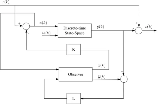
Observer L + -+ -Discrete-time State-Space K +
-Figure 6.1 Linear state-space model (linmod) of the system with reference
The mathematical model of the system is described by the following ordinary differential equations:
(6.1)
Here, the states of the system, and denote biomass concentrations and and denote substrate concentrations. The disturbance, which is the influent concentration, is denoted with . The dilution rate, , is chosen as the control input. The specific growth rate of the microorganisms, , is defined to be as
(6.2)
The methane flow rate, is the measurable output and defined to be as:
(6.3) The parameters of the anaerobic system to be controlled are presented in Table 6.1. The values at the operating points, where the linearization process is performed are selected
as follows, and .
Table 6.1 The parameters of the anaerobic system
0.2 0.25 0.3 0.87 6.7 4.2 5 4.35
The linearization procedure is given in detail in the Ref. [53]. After some straight forward calculations the linearized state-space model can be obtained as follows:
(6.4) As explained with a flow diagram shown in Figure 6.2, first, the minimum is computed for problem with no constraint. We obtain . The parameter for bounding the disturbance was selected as and consequently is obtained. In this case, the control input is constrained as .
Solve the LMI (4.7), according to given α0
and r0 values while ξ=x(0)=0 by using initial
conditions. Then calculate K and P values. Step1: Assign r=r0 for k=0; Step2: K0=K P0=P p0=0
Solve LMI (4.7) for ξ=x(0). Is there any possible solution?
x(0)=0 x(0)≠0
Yes No
Calculate
K0, P0, p0
Increase r
At step k, obtain the control signal u(k)=Kkx(k) by using
the calculated value of Kk. Then calculate the next State
by x(k+1)=Ax(k)+Buu(k)+Bww(k). Any possible
solution? Yes No Calculate Kk, Pk, pk Increase r Step3:
During the control experiments, first, a PID control is applied to the system. The PID coefficients that make the controller performance optimum were obtained by means of the Ziegler-Nichols method given in [54] and provided in Table 6.2.
Table 6.2 The PID coefficients computed by means of Ziegler-Nichols method.
2.23 0.98 1.32
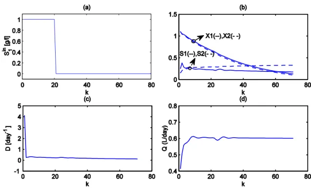
A step type disturbance input, as shown in Figure 6.3 (a), is applied to the system controlled with the PID controller. The variation of the states of the system under the PID control is presented in Fig. 6.3 (b).
Figure 6.3 PID control of the anaerobic system (a)Disturbance , (b) bacteria growth curves in the reactors, , and substrate levels , (c) control input,
(d) methane gas output .
Figure 6.3 (c) shows the time-history of the control signal. It is practically obtained through an input valve, which manipulates the dilution rate, D. Due to the effect of integral term of the PID controller, the methane gas output reaches the desired level in a reasonably short time as seen in Figure 6.3 (d). However, it should be noted that the PID coefficients computed are valid only for the operating point taken into consideration.
Then, as a second case, the system of interest is controlled first with the classical controller followed by the moving horizon controller. The simulation results obtained from these two control approaches are plotted in the same graph as shown in Figure 6.4. For this case the same disturbance signal is used as in the previous case. The variation of the in the state variables of the first and the second reactor are shown in Figure 6.4 (a) and Figure 6.4 (b), respectively. The energy of control signals are shown in Figure 6.4 (c) and the variation of the methane gas outputs are depicted in Figure 6.4 (d). The methane gas outputs produced by applying the moving horizon and classical controls to the system are plotted in the same graph for a fair comparison as shown in Figure 6.4 (d). It is easy to see that, MHHC method allows us to obtain much better control performance when compared to those obtained by using classical method. This is reasonable because the optimization is performed at each step of run-time instead of an off-line design. Furthermore, the energy of the control signal used for the moving horizon control is found to be smaller compared to the classical control, as clearly indicated in Figure 6.4 (c). Thus, it is concluded that moving horizon
control has yielded satisfactory results.
Figure 6.4 Moving horizon control (− −) vs. control (─) on (a) State variables of the first reactor, (b) state variables of the second reactor, (c)
Example 2:
The following example is borrowed from [41] in which a nominal control problem has been considered. Consider a state-delayed system (5.1) whose model parameters are given by
Choosing , and using the energy bounded disturbance whose time-history is as shown in Figure 6.5, we compute for at the initial step of Algorithm1. Applying the proposed algorithm on the system we obtain satisfactory results in minimization which also leads us to obtain a significant improvement in disturbance rejection performance. Fig. 6.6 shows the changes in with respect to delay bounds. On the other hand, Table 6.3 provides the values at each step.
Table 6.3 values at each step in Example 2 1 2-40 41 42-48 49-50 51-58 0.3 0.4 0.6 0.7 0.75 0.45
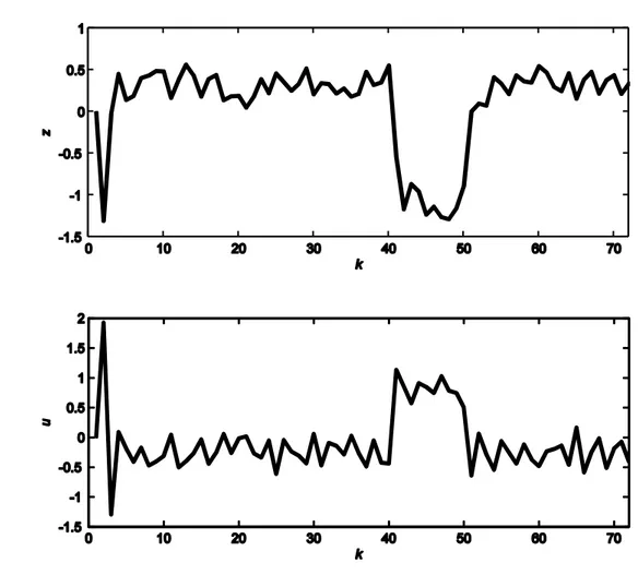
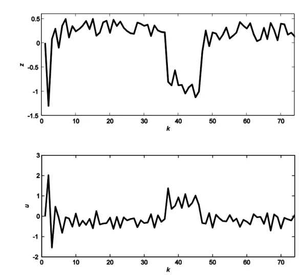
For different delay bounds, and the variation of the controlled output, and the control signal, are shown in Figure 6.7, Figure 6.8, Figure 6.9 and Figure 6.10.
Figure 6.7 The time-history of the controlled output, , and control input, , for .
Figure 6.8 The time-history of the controlled output, , and control input, , for .
Figure 6.9 The time-history of the controlled output, , and control input, , for .
Figure 6.10 The time-history of the controlled output, and control input, for .
Example 3: We utilize the example given in Ref. [17] in revised form as follows:
where .
The time-history of the disturbance applied to the system is as shown in Figure 6.5. During the simulations, the best variation of is obtained as given in Table 6.4. Figure 6.11 shows the variations in with respect to different delay-bounds. For various delay bounds, and , we obtain the time-history of performance outputs and the control efforts as shown in Figure 6.12, Figure 6.13 and Figure 6.14.
The disturbance signal applied to the system is as shown in Figure 6.5. During the simulations, the best variation of is obtained as given in Table 6.4. Figure 6.11 shows the variations in with respect to different delay-bounds. For various delay bounds, and , we obtain the time-history of performance outputs and the control efforts as shown in Figures 6.12, 6.13 and 6.14.
Table 6.4 values at each step in Example 3. 1 2-40 41 42-48 49-50 51-58 0.3 0.4 0.6 0.7 0.75 0.45
Figure 6.11 The variations of disturbance attenuation level, , for different delay intervals.
Figure 6.12 The time-history of the controlled output, , and control input, , for .
Figure 6.13 The time-history of the controlled output, , and control input, , for .
Figure 6.14 The time-history of the controlled output, , and control input, , for .
CHAPTER 7
CONCLUSIONS The MHHC of a class of linear discrete-time, uncertain time-delayed systems having time-varying interval delays was considered. Utilizing a standard discrete-time Lyapunov-Krasovskii functional, some delay dependent, Linear Matrix Inequality (LMI) based conditions which need to be solved iteratively in each step of run-time were provided. The provided LMI based conditions guarantee the closed-loop asymptotic stability, maximum disturbance attenuation performance and closed-loop dissipativity in consideration of the physical limitations of the actuator. The dissipation constraint that is utilized to guarantee closed-loop system dissipativity and performance is less conservative than requiring monotonicity of the value function. The proposed MHHC has a capability of taking the performance criterion into account, while some of other stabilizing state-feedback controls for time-delay systems can only achieve stability. On the other hand, the proposed algorithm comes with a computational burden that complicates the real-time applications. To overcome this problem, certain calculations can be carried out offline, which can be stated as a future study on MHHC for time-delay systems.
Three numerical examples which consist of nominal and uncertain system models were considered to demonstrate the applicability of the proposed approach. Both the numerical results and simulation results validated that the proposed approach of this note can be efficiently used for the control of discrete-time, time-delayed systems having uncertainties and physical control limitations.
For a further study, the conservatism of the approach can be alleviated by using complete L-K functional and/or some delay-decomposition methods. However, it is probable that both strategies would impose noticeable amount of additional computational loads to the controller which will prohibit the use of the proposed method
in real-time. Also these types of methods cannot be solved by using convex optimization methods and would require the use of some linearization techniques such as cone-complementary methods. Extension of the proposed results to time varying delayed systems with input constraint is also considered to be a future work.
REFERENCES
[1] Mahmoud, M.S., (2000). Robust Control and Filtering for Time-Delay Systems. Marcel Dekker Inc.: New York.
[2] Gu, K., Kharitonov, V. and Chen, J., (2003). Stability of Time Delay Systems. Birkhauser: Basel, Boston.
[3] Moon, Y.S., Park, P., Kwon, W.H. and Lee, Y.S., (2001). "Delay-dependent robust stabilization of uncertain state-delayed systems", International Journal of Control, 74:1447–1455.
[4] Richard, J.P., (2003). "Time-delay systems: an overview of some recent advances and open problems", Automatica, 39:1667–1694.
[5] De Souza, C.E. and Li, X., (1999). "Delay-dependent robust control of uncertain linear state-delayed systems", Automatica, 35:1313–1321.
[6] Peng, C., Yue, D. and Tian, Y.-C., (2009). "New Approach on Robust Delay-Dependent Control for Uncertain T-S Fuzzy Systems with Interval Time-Varying Delay", IEEE Transactions on Fuzzy Systems, 17:890–900.
[7] Parlakçı, A. and Küçükdemiral, I.B., (2011). "Robust delay-dependent control of time-delay systems with state and input delays", International Journal of Robust and Nonlinear Control, 21:974–1007.
[8] Niculescu, S.-I., (1998). " Memoryless Control with an α-Stability Constraint for Time-Delay Systems: An LMI Approach", IEEE Transactions on Automatic Control, 43:739–743.
[9] Fridman, E. and Shaked, U., (2002). "An improvement stabilization method for linear time-delay systems", IEEE Transactions on Automatic Control, 47:1931– 1937.
[10] Suplin, V., Fridman, E. and Shaked, U., (2006). " Control of Linear Uncertain Time-Delay Systems-A Projection Approach", IEEE Transactions on Automatic Control, 51:680–685.
[11] Peng, C. and Tian, Y.-C., (2009). "Delay-dependent robust control for uncertain systems with time-varying delay", Information Sciences, 179:3187– 3197.
[12] Li, H., Chen, B., Zhou, Q. and Lin, C., (2009). "A Delay-Dependent Approach to Robust Control for Uncertain Stochastic Systems with State and Input Delays", Circuits Syst Signal Process, 28:169–183.
[13] Jiang, X. and Han, Q.-L., (2005). "On Control of Linear Systems with interval time-varying delay", Automatica, 41:2099–2106.
[14] Xiao, M. and Shi, Z., (2009). "Delay-Dependent Guaranteed Cost Control of an Interval System with Interval Time-Varying Delay", Journal of Inequalities and Applications, 1–16.
[15] Yan, H., Zhang, H., Meng, M.Q.-H. and Shi, H., (2010). "Delay-range-dependent robust filtering for uncertain systems with interval time-varying delays", Asian Journal of Control, 13:356–360.
[16] Tian, E., Yue, D. and Zhang, Y., (2011). "On improved delay-dependent robust control for systems with interval time-varying delay", Journal of the Franklin Institute, 348:555–567.
[17] He, Y., Wu, M., Han, Q.-L. and She, J.-H., (2008). "Delay-dependent control of linear discrete-time systems with an interval-like time-varying delay", International Journal of Systems Science, 39:427–436.
[18] Caldeira, A.F., Leite, V.J.S., Miranda, M.F., Castro, M.F.F. and Goncalves, E.N., (2011). "Convex robust control design to discrete-time systems with time-varying delay", Proceedings of the 18th IFAC World Congress, Milano, Italy. 10150–10155.
[19] Rawlings, J.B., (2000). "Tutorial overview of model predictive control", Control Systems, IEEE, 20:38–52.
[20] Bemporad, A., Borrelli, F. and Morari, M., (2002). "Model predictive control based on linear programming~ the explicit solution", IEEE Transactions on Automatic Control 47.12: 1974-1985.
[21] Magni, L., Nicolao, G. De, Scattolini, R. and Allgöwer, F., (2003). "Robust model predictive control of nonlinear discrete-time systems", International Journal of Robust and Nonlinear Control, 13:229–246.
[22] Wan, Z. and Kothare, M. V., (2003). "An efficient off-line formulation of robust model predictive control using linear matrix inequalities", Automatica, 39:837– 846.
[23] Kwon, W.H. and Han, S., (2005). Receding horizon control: model predictive control for state models. Springer.
[24] Camacho, E.F. and Bordons, C., (2004). Model predictive control. Springer London.