c
⃝ T¨UB˙ITAK
doi:10.3906/elk-1304-210 h t t p : / / j o u r n a l s . t u b i t a k . g o v . t r / e l e k t r i k /
Research Article
An E-Nose-based indoor air quality monitoring system: prediction of combustible
and toxic gas concentrations
Bekir MUMYAKMAZ1,∗, Kerim KARABACAK2
1
Department of Electrical and Electronics Engineering, Dumlupınar University, K¨utahya, Turkey
2K¨utahya Technical Sciences Vocational School, Dumlupınar University, K¨utahya, Turkey
Received: 22.04.2013 • Accepted/Published Online: 24.05.2013 • Printed: 30.04.2015
Abstract: A system for monitoring and predicting indoor air quality level is proposed in this paper. The system comprises a computer with a monitoring program and a sensor cell, which has an array of metal oxide gas sensors along with a temperature and humidity sensor. The gas sensors in the cell have been chosen to detect only hydrogen, methane, and carbon monoxide gases. Methane was selected as a representative for indoor combustible gases, and carbon monoxide was used to represent indoor toxic gases. Hydrogen was used as an interfering (and also combustible) gas in the study. A number of experiments were conducted to train the three artificial neural networks of the monitoring system. The networks have been trained using 80% of the gathered data with the Levenberg–Marquardt algorithm. The results of this work show that the performance rate of the proposed monitoring system in determining gas type for the limited sample space is 100% even when there is an interfering gas such as hydrogen in the environment. The trained system can predict the concentration level of the methane and carbon dioxide gases with a low absolute mean percent error rate of almost 1%.
Key words: Electronic nose, E-Nose, air quality monitoring, artificial neural networks
1. Introduction
Indoor air pollution is a significant and growing health concern. Respiratory infections, asthma, and lung cancer are well-known effects of air pollution. It is the cause of more than a million human deaths globally, accounting for nearly 5% of the worldwide death rate in 2000 [1]. The sources of air pollution in homes include combustion sources such as coal, wood, oil, and gas; building materials and furnishings; products for household cleaning; and central heating and cooling systems. These are responsible for the emissions of carbon monoxide (CO), radon, and volatile organic compounds (VOCs). Other sources of air pollution in any home are carbon dioxide (CO2) (mainly emitted by humans), particulates, and microbial contaminants such as mold and bacteria.
There is an increasing interest in indoor air quality (IAQ) monitoring since building-related illnesses and syndromes are growing mainly due to long-term occupancy in limited living spaces. Parra et al. studied the seasonal variability of VOCs in pubs and cafes [2]. Exposure of school-aged children to specific pollutants such as sulfur dioxide (SO2) , CO, and nitrogen dioxide (NO2) in Western Europe and North America was reviewed by Ashmore and Dimitroulopoulou [3]. Yu et al. proposed a wireless sensor network system to monitor carbon dioxide concentration [4]. Seasonal models for monitoring and predicting IAQ in subway or metro systems were developed by Kim et a.l [5].
In modern systems, IAQ monitoring is provided by an electronic nose (E-Nose). It was defined in 1994 by Gardner as an instrument that comprises an array of electronic chemical sensors and an appropriate pattern-recognition system and it is capable of recognizing both simple and complex odors [6]. Many types and uses of electronic noses have been reported in the literature. A review paper on the electronic nose applied to dairy products was presented by Ampuero and Bosset [7]. Kateb et al. investigated the possible usage of an electronic nose to distinguish two types of tumor cells [8]. Metal oxide gas sensor modeling by neural networks to decrease the risk of false alarms and missed detections was proposed by Hakim and Zohir [9].
In this study, an E-Nose device design based on a metal oxide gas sensor array for the classification and the quantification of two gases is presented. The concentration ranges of the gases were selected to be compatible with IAQ monitoring purposes. Carbon monoxide was selected as a toxic gas and methane was selected to represent combustible gases. Hydrogen, which is also a combustible gas, was chosen as an interfering type, since metal oxide gas sensors respond well to H2. The gas sensors and their driving electronics circuitry were used to capture and send the IAQ data to the monitoring system, which comprised a personal computer (PC) and a piece of software developed in this study. The sensor array consisted of a humidity and temperature sensor and three chemical gas sensors. A pattern recognition algorithm, based on an artificial neural network (ANN), was run and a graphic user interface (GUI) program showed the concentrations of the above-mentioned gases simultaneously with their changes over time on the screen.
The main objectives of this study are to show abilities of the proposed E-Nose in terms of IAQ and to study the incidence of the interfering gas in the indoor air samples with the gas sensors.
2. Experiment
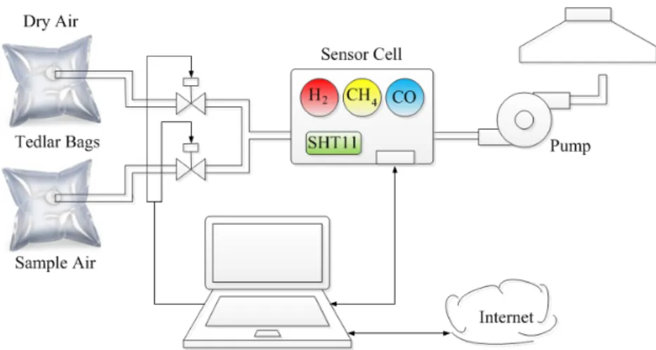
The experimental setup is shown in Figure 1. The sensor cell has an array of gas sensors, a humidity and temperature sensor, and their driving electronics including a microcontroller. The gases contained in the Tedlar bags are delivered via computer-controlled valves to the sensor cell using a small pump. The gathered data in the microcontroller are then sent to a PC that has a suitable pattern recognition algorithm and a monitoring program. The data are then visualized on the screen in real time and processed in order to determine the concentration of the constituent gas amounts in the mixture.
Figure 1. Basic configuration of the experimental system.
The target gases in the study are methane (CH4) , carbon monoxide (CO), and hydrogen (H2) . Carbon monoxide is a toxic gas. It is also colorless and odorless. Higher concentrations of CO exposure can be very
dangerous, even fatal. Average levels of carbon monoxide in homes without gas stoves vary from 0.5 to 5 ppm. However, levels may be 30 ppm or higher in homes that have poorly adjusted stoves (www.epa.gov/iaq/co.html). Recommended exposures have been restricted to as low as 100 mg/m3 (87 ppm) for 15 min or 30 mg/m3 (26 ppm) for 1 h by the World Health Organization (www.who.int/ipcs/publications/ehc/ehc 213/en/). An additional property of carbon monoxide is its flammability. The lower explosive limit (LEL) for CO is 12%.
Hydrogen (LEL: 4%) and methane (LEL: 5%) gases are flammable and also odorless and colorless like CO, but they are not toxic, only asphyxiants. High concentrations of these gases cause dizziness, possible nausea, and eventual unconsciousness by blocking the adequate supply of oxygen to the lungs. Small natural gas leaks (mostly methane) may not be considered as common air pollutants, but they are indeed a threat for human life because they cause oxygen deficiency even if they do not cause an explosion.
The concentration ranges of the target gases in the carrier gas (dry air) were determined as 25–500 ppm for H2, 25–750 ppm for CO, and 400–10,000 ppm for CH4 in this study. The concentrations were well below the LEL of each gas since the purpose of the study was to monitor IAQ. The Tedlar bags (12 L) in Figure 1 were filled with 10 L of dry air using mass flow controllers. The necessary concentrations of gas mixtures were achieved by using 2.5-mL and 50-mL syringes. The sample gas and the dry air (as a purging gas) were alternately sent to the sensor cell with a fixed flow rate of 200 cm3/min by a small pump as shown in the figure. Metal oxide semiconductor-based gas sensors made by Figaro Company were used in the E-Nose. The resistances of these sensors change with the presence of a target gas. The output voltages of the sensors also change since they behave like a voltage divider. After the sample gas was introduced to the sensors, the output voltage changes of the sensors were sampled and forwarded to the PC by a microcontroller (PIC from Microchip). The microcontroller has a 10-bit analog-to-digital converter (ADC), so a voltage input of 5 V corresponds to the number of 1024 as the ADC number in the chip. The sensors were chosen to detect within the range of the above-mentioned concentration rates, as shown in Table 1. Although the room temperature was kept at around 23 ◦C and dry air was used during the experiments, the temperature and humidity in the sensor cell were recorded by the humidity and temperature sensor (SHT11 by Sensirion AG).
Table 1. Metal oxide gas sensors and their typical detection ranges.
Sensor Target gas Typical detection range
TGS2611 Methane 500–10,000 ppm
TGS821 Hydrogen 10–4000 ppm
TGS2442 Carbon monoxide 30–1000 ppm
In order to calibrate the E-Nose, a number of experiments were conducted. First, voltage gains of the sensors were maximized in their detection ranges. Each sensor was then tested for its repeatability. The numbers, types, and concentration values of the experiments for calibration are illustrated in Figure 2. The sample bags related to individual gas compositions were prepared in 10 different concentration levels of each gas in dry air. The other samples included binary mixtures of CO and CH4 in the carrier gas as shown in Figure 2. The CH4 gas concentrations in mixture samples were arranged in the levels of 2000, 3000, and 4000 ppm. The concentration level of the CO was changed in 5 steps for each CH4 level of experiments starting from 100 to 500 ppm in 100 ppm increments.
0 5 10 15 20 25 30 35 40 45 0 100 200 300 400 500 600 700 800 900 1000 Co n ce nt rations (ppm) 0 5 10 15 20 25 30 35 40 450 1000 2000 3000 4000 5000 6000 7000 8000 9000 10000 Sample Number Con ce nt rations (ppm) Methane Hydrogen Carbon Monoxide
Figure 2. Experiments in the calibration process of the E-Nose.
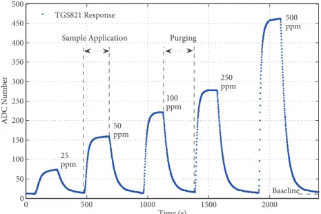
The measurements were made three times for each prepared sample as shown in Figure 2. The E-Nose was run first for 15 min without any gas application. Purging gas (dry air) was then applied for 15 min to settle the baseline of the sensors prior to measurements. Five sample bags were prepared for measurements related to the 5 steps in Figure 2 and alternately sent with dry air to the sensor cell. This type of measurement is called a purged measurement. One example of this is shown in Figure 3. There were five different concentration levels of hydrogen in dry air as shown. After purging, a sample gas was applied to the sensor cell. The sensor response eventually increased and reached a steady state level as shown. Figure 3 does not show the actual voltage changes of the sensor; instead, it shows the corresponding analog-to-digital converter numbers (ADC numbers). The difference between the baseline and the steady-state level was calculated as an indication of the H2concentration in the sample bag.
0 500 1000 1500 2000 0 50 100 150 200 250 300 350 400 450 500 Time (s) ADC N umber TGS821 Response
Sample Application Purging
250 ppm 100 ppm 50 ppm 25 ppm 500 ppm Baseline
Figure 3. TGS821 sensor responses to five different H2 concentrations with purging.
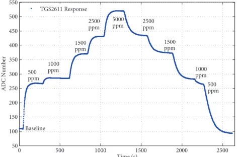
The second type of measurement was made without purging. For this kind of measurement, five sample bags were prepared again for measurements related to the 5 steps in Figure 2, but the samples were sent
consecutively in increasing and decreasing order to the sensor cell without purging (see Figure 4). The TGS2611 sensor response to methane, which had changing concentration in 5 steps, is shown in Figure 4. The sensor steady-state response for the same concentration of methane (e.g., 1500 ppm) in Figure 4 is almost equal and shows the repeatability of the sensor.
0 500 1000 1500 2000 2500 50 100 150 200 250 300 350 400 450 500 550 Time (s) ADC N umber TGS2611 Response 500 ppm Baseline 500 ppm 1000 ppm 1500 ppm 2500 ppm 5000 ppm 2500ppm 1500 ppm 1000 ppm
Figure 4. TGS2611 sensor responses to five different CH4 concentrations without purging.
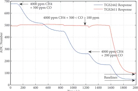
Responses of the TGS2611 and TGS2442 sensors to binary gas mixtures of CH4 and CO in dry air are shown in Figure 5. The concentration level of CH4 was kept constant at 4000 ppm while the concentration level of CO was changing in 5 steps, starting from 500 ppm and decreasing by 100 ppm in each step. There were no purging gas applications during the experiment. The response of the methane sensor was almost constant since the concentration level of methane in the sample bags had been chosen constant at 4000 ppm. However, the response of the other sensor was decreasing gradually depending on the concentration level of the carbon monoxide gas in the sample bag. At the end, the responses of the sensors returned to their baseline levels with the application of dry air. Thus, the sensors reacted selectively. The differences between the steady state responses and the baseline levels of the sensors were saved and used for calibrating the system.
There were 3 different gases in 10 concentrations in the individual gas experiments. The number of binary gas mixtures with 5 different concentrations of CO in each was 3. The experiments were made with purging, without purging in increasing order, and without purging in decreasing order. Thus, the total number of the conducted measurements for calibration was (3 × 10 + 5 × 3) × 3 = 135. In order to avoid possible noise and experimental errors, only the mean values of the equivalent measurements related to the same amount of gas compositions were used for calibrating the networks. The baseline response level measurement, which corresponded to a no-gas medium other than dry air, was then also added to the dataset. Thus, the dataset was obtained as (135 / 3) + 1 = 46.
3. Data processing and calibration process
The differences between the steady-state responses and the baseline levels of the gas sensors were applied to the data processing unit and a concentration prediction was made for each target gas in dry air. The unit extracted
information from the experimental data using a nonlinear method comprising 3 stages, namely normalization, denormalization, and ANN. Figure 6 shows the internal details of the data processing unit. The input values of the processing unit were converted into the range of 0 and 0.9 in the normalization block. The normalized values were fed into the trained ANNs, and the outputs of the networks (which were again in the range of 0 and 0.9) were converted to the concentration ppm levels in the denormalization block. There were three ANNs in this study, each of which predicted only one type of gas concentration level.
0 200 400 600 800 1000 1200 1400 1600 1800 2000 0 100 200 300 400 500 600 700 Time (s) ADC N umber TGS2442 Response TGS2611 Response 4000 ppm CH4 + 200 ppm CO 4000 ppm CH4 + 500 < CO > 100 ppm 4000 ppm CH4 + 500 ppm CO Baselines
Figure 5. TGS2611 and TGS2442 sensor responses to five different CO concentrations mixed with 4000 ppm CH4.
Figure 6. Data processing unit for concentration prediction.
Each ANN block in Figure 6 has a multilayer feedforward neural network with one input, one hidden, and one output layer. There were 3 inputs in the input layer of the networks since the number of gas sensors was 3 in the system. The number of neurons in the hidden layer of each network was determined as 7 by trial and error. The output layer of each network had only one neuron because each network predicted only one type of gas concentration. Thus, the architecture was 3-7-1 for each network. Activation functions of the neurons in the ANNs were selected as a logarithmic sigmoid since the inputs and the outputs were in the range of 0
and 0.9. The weights and biases of the networks were adjusted to fulfill the necessary nonlinear relationship between the inputs and the outputs by using a training algorithm [10].
The network topology did not change during the training. The weights and biases were iteratively updated to minimize the network performance function. The performance function was chosen as mean squared error in this study. The weights and biases of the network were updated after the whole training dataset was applied to the network since batch mode training was used. The gradients calculated at each training example were added together to determine the changes in the weights and biases [11].
The total collected number of samples in the dataset was 46 in the study. The dataset was divided into 3 subsets as training, validation, and testing [12]. Since the number of samples was very limited, only one arbitrarily selected sample related to each individual gas measurement was added to the validation subset. The same selection process was also done for the testing subset. Two samples for the validation subset and one sample for the testing subset were chosen from the mixture of CO and CH4 measurements. Thus, the total number of samples for the validation and testing subsets was 9, corresponding to 20% of total samples. The remaining 37 samples (80%) were used for training.
There are many training algorithms for multilayer feedforward networks. For curve-fitting or function approximation problems such as that in our study, the Levenberg–Marquardt algorithm can converge faster than the others for networks that contain up to a few hundred weights according to the results of several studies [13]. The algorithm is capable of obtaining lower mean square errors in many cases. Since the architecture is 3-7-1 for each network, there are only (3 × 7) + 7 = 28 weights in each network. Thus, the Levenberg– Marquardt algorithm was used in this study. All calculations and programming were done using MATLAB from MathWorks.
4. Results and discussion
The number of target gases was 3 and there were also 3 gas sensors used in the study. Since there were nonlinear relationships between the sensor responses and the corresponding gas concentrations, it was necessary to use nonlinear mapping between the inputs and the outputs in a multivariable space. Thus, ANNs were chosen to be used to obtain the solution of the problem. The neural network architecture could have been created with 3 inputs, 3 outputs, and a hidden layer with a satisfactory number of neurons, and then only one ANN would be sufficient for predicting concentrations of the target gases. However, the training of the ANN would have been very difficult with the limited number of collected samples in the study. Therefore, the number of ANNs was decided to be 3, with 3 inputs, 1 output, and a hidden layer with a sufficient number of neurons. The optimum numbers of neurons in the hidden layers of the ANNs were decided by trial and error. The final data processing unit comprised 3 ANNs that were identical in the network architecture of 3-7-1. Each network was individually trained to predict the concentration of a certain gas.
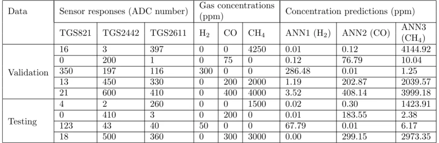
The validation and testing data for the ANNs are shown in Table 2. The training dataset has not been included in the table to limit the size. The sensor responses were very selective for CO and CH4, but all of the sensors also responded to H2 as expected. The first ANN, which was related to the hydrogen gas concentration prediction, achieved a performance level of 1.18 × 10⁻⁶ mean squared error (MSE) in 13 epochs for training data and 1.18 × 10⁻⁴ MSE for validation data. The validation data were not used in the training of the network, but they were used to sense the possible overfit problem in the learning process and to find the epoch number of the optimum solution.
product of their standard deviations. It is a measure of the strength of linearity between those variables and can be used to test the generalization ability of a trained network. The R-values between the network outputs and the corresponding real output values were almost 1 for ANN1. Similar achievements were also obtained for the other two networks. The concentration prediction results of the networks are presented in Table 2. MSE and R-values are shown in Table 3.
Table 2. The validation and testing data for the ANNs.
Data Sensor responses (ADC number) Gas concentrations Concentration predictions (ppm) (ppm)
TGS821 TGS2442 TGS2611 H2 CO CH4 ANN1 (H2) ANN2 (CO) ANN3
(CH4) Validation 16 3 397 0 0 4250 0.01 0.12 4144.92 0 200 1 0 75 0 0.12 76.79 10.04 350 197 116 300 0 0 286.48 0.01 1.25 13 450 330 0 200 2000 1.19 202.87 2039.57 21 600 410 0 400 4000 3.52 408.14 3999.18 Testing 4 2 260 0 0 1500 0.02 0.30 1423.91 0 410 3 0 200 0 0.01 183.55 2.38 123 43 40 50 0 0 67.79 0.01 6.17 18 500 360 0 300 3000 0.00 299.15 2973.35
Table 3. ANNs and their training results.
Network ANN1 ANN2 ANN3
Training MSE 1.18× 10⁻⁶ 3.88× 10⁻⁶ 3.75× 10⁻⁶ Validation MSE 1.18× 10⁻⁴ 2.24× 10⁻⁵ 2.06× 10⁻⁵ R-Value (training) 0.99999 0.99997 0.99998 R-Value (validation) 1 0.99998 0.99997 R-Value (testing) 1 0.99864 0.99974 R-Value (overall) 0.99947 0.99987 0.99994
The MSE and R-values in Table 3 show the level of the generalization ability of the networks for the dataset. The MSE values are sufficiently low for both the training and validation dataset. The R-values are almost 1 for the training, validation, and testing datasets. It can thus be concluded that there is no under- or overfitting problem in the training phase of the networks. Another way of describing the performance of the networks is to give absolute percent errors. The absolute percent error formula is:
|%e| = Tv− Pv Tv × 100.
(1)
The mean absolute percent error (MAPE) is:
M AP E = 1 n n ∑ v=1 Tv− Pv Tv × 100, (2)
where Tv is the actual target value, Pv is the predicted value, and n is the number of total calculated absolute
percent errors.
Table 4 presents the mean (MAPE), median, and maximum absolute percent errors of the networks. The individual percent errors of the predictions are again not included due to space considerations. Individual
percent errors for validation and testing data can easily be calculated from the data provided in Table 2. The mean and median errors are considerably lower than the maximum error values in Table 4. The maximum error values can be classified as outliers since their quantities are so small in the whole of the data. The biggest error was recorded as 35.59% in Table 4 since the target value was 50 ppm of H2 (very low concentration) and the corresponding prediction value of ANN1 was 67.79 ppm. This error could be decreased by using more samples in the training phase of the networks. The last column of Table 4 shows the absolute mean, median, and maximum percent error values of the total sample space.
Table 4. The absolute percent error values (|e%|) in predictions of ANNs.
Network Training samples Validation samples Testing samples All samples
(|e%|) (|e%|) (|e%|) (|e%|)
ANN1 Mean 0.21 0.90 8.90 1.04 Median 0.00 0.00 0.44 0 Max. 2.97 4.51 35.59 35.59 ANN2 Mean 0.64 1.17 2.13 0.83 Median 0.02 1.44 0.14 0.02 Max. 6.23 2.40 8.22 8.22 ANN3 Mean 0.55 0.89 1.49 0.67 Median 0.06 0.02 0.44 0.04 Max. 3.23 2.47 5.07 5.07
The percent error rates can be used as an indicator for the quantitative performance rate of the system. The mean and median percent error values are lower than or close to 1% in Table 4. Thus, the system is quantitatively very successful at predicting the gas amounts. On the other hand, the qualitative performance rate of the system can be defined according to the percentage of correct classifications of the system for the sample space. If the outputs of the system are below the sensitivity range of the sensors, that means there is no target gas in the environment. Otherwise, there is a target gas in the environment. If the target and predicted gas concentration data in Table 2 are examined in this sense with the help of information in Table 1, it can be concluded that the qualitative performance rate of the system is 100% for the validation and testing data. The same result is also true for the training data.
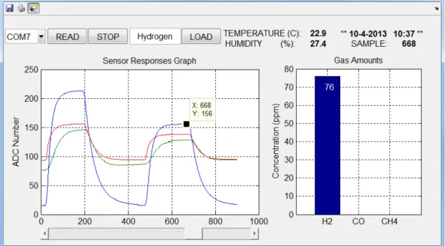
The network structures and their parameters were put into a graphical user interface program after offline training. The program could read, save, load, and visualize the sensor data as needed. When the prerecorded sensor data were loaded, the program calculated the difference between the baseline and the sensor readings at the time of the slider position. These values were then sent to the ANNs for concentration prediction. The outputs of the networks were visualized as a bar plot in the program. An example of sensor array data is visualized in Figure 7. The data were related to the measurements of 100 and 75 ppm of hydrogen in dry air. Hydrogen could be considered as both the target and interfering gas for the system. Although there was no gas present other than hydrogen in this example, all sensors responded to the sample gas. However, the monitoring system showed only the presence of hydrogen gas. At the 668th second from the beginning of the measurement, the H2 level was shown as 76 ppm on the bar plot, while the corresponding real value of the hydrogen concentration of the sample bag was 75 ppm and there was no other gas.
Air quality monitoring with the proposed system can be started with the application of a purging gas. The response levels of the sensors were used as baseline levels after 5 to 10 min, and then the target gases could be applied. Immediately after the sample bag was applied to the system, sensor readings were seen on the screen and the possible target amounts were determined. Figure 8 shows the results of an experiment with five
different binary gas mixtures of CH4 and CO in dry air. The CH4 concentration levels in the sample bags were kept at 2000 ppm and the CO concentration levels in the sample bags were changed in increasing order from 100 ppm to 500 ppm. The last sample bag had 2000 ppm CH4 and 500 ppm CO in dry air. The monitoring system indicated very close readings and predicted the concentration levels of 0 ppm for H2, 535 ppm for CO, and 2018 ppm for CH4. Although the H2 sensor responded to the sample to some extent, the monitoring system showed the presence of only CO and CH4.
Figure 7. A screenshot from the air quality monitoring program.
The calibration process in this study was done with a very limited sample space and only for individual gas compositions of H2, CO, and CH4 and for binary mixtures of CO and CH4. The study can be extended to cover other gases related to air pollution. This requires increasing the number of experiments depending on the number of gases present in the mixture. Ternary gas mixtures of VOCs were studied in a previous work [14]. The experiments in this study were done in dry air conditions and do not cover humidity and temperature compensation. The sensors in the monitoring system are affected to some extent by the temperature and humidity of the medium. Calibration of the air quality monitoring system with the presence of humidity or temperature changes in the environment can be done by conducting more experiments. Such a task was done in a previous study [15].
The proposed system was designed and trained only for 3 combustible and/or toxic gases. The number of target gases could be further extended by changing and retraining the ANNs of the system even without adding more sensors since gas sensors might respond to any gas in the environment to some degree.
5. Conclusion
In this study, an E-Nose-based IAQ monitoring system was introduced. The system utilized the sensor array responses and predicted the concentration levels of hydrogen, methane, and carbon monoxide in the environment. The ANNs of the monitoring system were trained with the Levenberg–Marquardt algorithm using 80% of the conducted experiments. The study results showed that the qualitative performance rate of the system on correct classification of the species was 100% and the system could determine the presence of the target gases without being affected by interfering gas. The quantitative performance rate of the system was also very promising, with a MAPE of as low as 1% for the limited sample space, and it could be improved by conducting more experiments. The number of the target gases for air quality monitoring could be increased by using more sensors and/or retraining the ANNs in the system. Compensation for drifts in the sensors caused by humidity and temperature changes in the environment could also be made by retraining the ANNs of the monitoring system.
Acknowledgment
This work was supported by Dumlupınar University (No: 2010-10).
References
[1] Ezzati M, Kammen DM. The health impacts of exposure to indoor air pollution from solid fuels in developing countries: knowledge, gaps, and data needs. Environ Health Persp 2002; 110: 1057–1068.
[2] Parra MA, Elustondo D, Bermejo R, Santamaria JM. Quantification of indoor and outdoor volatile organic com-pounds (VOCs) in pubs and caf´es in Pamplona, Spain. Atmos Environ 2008; 42: 6647–6654.
[3] Ashmore MR, Dimitroulopoulou C. Personal exposure of children to air pollution. Atmos Environ 2009; 43: 128–141.
[4] Yu TC, Lin CC, Chen CC, Lee WL, Lee RG, Tseng CH, Liu SP. Wireless sensor networks for indoor air quality monitoring. Med Eng Phys 2013; 35: 231–235.
[5] Kim M, Sankara Rao B, Kang O, Kim J, Yoo C. Monitoring and prediction of indoor air quality (IAQ) in subway or metro systems using season dependent models. Energ Buildings 2012; 46: 48–55.
[6] Gardner JW, Bartlett PN. A brief history of electronic nose . Sensor Actuat B-Chem 1994; 18: 210–211.
[7] Ampuero S, Bosset JO. The electronic nose applied to dairy products: a review. Sensor Actuat B-Chem 2003; 94: 1–12.
[8] Kateb B, Ryan MA, Homer ML, Lara LM, Yin Y, Higa K, Chen MY. Sniffing out cancer using the JPL electronic nose: a pilot study of a novel approach to detection and differentiation of brain cancer. NeuroImage 2009; 47: T5–T9.
[9] Hakim B, Zohir D. Enhancement of the neural network modeling accuracy using a submodeling decomposition-based technique, application in gas sensor. Neural Comput Appl 2012; 21: 1981–1986.
[10] Patterson DW. Introduction to Artificial Intelligence and Expert Systems. Englewood Cliffs, NJ, USA: Prentice Hall, 1990.
[11] Hagan MT, Demuth HB, Beale MH. Neural Network Design. Boston, MA, USA: PWS Publishing, 1996. [12] Haykin SS. Neural Networks: A Comprehensive Foundation. Englewood Cliffs, NJ, USA: Prentice Hall, 1999. [13] Hagan MT, Menhaj MB. Training feedforward networks with the Marquardt algorithm. IEEE T Neural Network
1994; 5: 989–993.
[14] Mumyakmaz B, ¨Ozmen A, Ebeo˘glu MA, Ta¸saltın C. Predicting gas concentrations of ternary gas mixtures for a predefined 3D sample space. Sensor Actuat B-Chem 2008; 128: 594–602.
[15] Mumyakmaz B, ¨Ozmen A, Ebeo˘glu MA, Ta¸saltın C, G¨urol ˙I. A study on the development of a compensation method for humidity effect in QCM sensor responses. Sensor Actuat B-Chem 2010; 147: 277–282.