Selçuk J. Appl. Math. Selçuk Journal of Vol. 9. No. 2. pp. 29 44 , 2008 Applied Mathematics
Some Comments on Solving Probabilistic Constrained Stochastic Programming Problems
Mehmet Y¬lmaz and Birol Topçu
Ankara University, Faculty of Science, Statistics Department, Ankara, Turkey e-mail: [email protected]
Afyon Kocatepe University, Faculty of Science and Literature, Department of Sta-tistics, Afyonkarahisar, Turkey
e-mail: [email protected]
Abstract. It is made some approaches for solving specialized probabilistic constrained stochastic programming problems (SPP). Since distribution of weighted sum can not be found exactly or formally or it has some di¢ culties in application, it is suggested that the usefulness of the normal approximation is called as …rst edgeworth series expansion for the probabilistic constrained SPP and related illustrative examples are given.
Key words: probabilistic constrained stochastic programming, weighted sum of random variates, …rst edgeworth series expansion
2000 Mathematics Subject Classi…cation. 60E05, 90C15, 62E17, 60E07 1. Introduction
Weighted sum of random variables is widely used in application areas of statistics such as weights selection in portfolio analysis, stock control, net-work system, etc. On the other hand, usually distribution of weighted sum
n P k=1
akXk can not be easily obtained. In literature, it is assumed that Xk’s have normal distribution, then it can be easily seen that
n P k=1
akXk is dis-tributed normal since normal distribution has in…nitely divisible distribution property. Otherwise for large n, applying the central limit theorem is preva-lent.
In the situation that the distribution of weighted sum can not be obtained easily or it has so complex structure such that it can not be used in appli-cations. Using the normal approximation named as …rst edgeworth series expansion and suggestion for solving probabilistic constrained are presented in this work. Along with that, three cases are considered for solving proba-bilistic constrained optimization problems. The …rst one is related to distri-bution of weighted stationary process, so that components are stochastically dependent. Second is also given for the dependent case, such that compo-nents are order statistics from exponential distribution. For the last case, it is considered that components are identically distributed and stochastically independent. For further discussions, explanatory examples are given. In section two, we will brie‡y give a de…nition of PCP which is one of the SPP. 2. Probabilistic Constrained Stochastic Models
In the case that whole model coe¢ cient or some of them are random, the problem is clearly SPP. If the technologic coe¢ cients on right side are random then the problem is called PCP. Simple probabilistic constrained model of which technologic coe¢ cients are random is as follows:
max(min)z(a) = n P j=1 cjaj n P j=1 xijaj ti i = 1; 2; :::; m aj 0 j = 1; 2; :::; n
if these constraints are changed with probabilistic constraints on the prede-…ned i probability levels, then the model is set up
(1) P n P j=1 Xijaj ti ! i i = 1; 2; :::; m
Here aj decision variables are deterministic, xij technologic coe¢ cients, ti right side, or cj may be random variables (see, Charnes and Cooper, 1959; Taha, 1997). One of the method of solving above problem is to obtain their deterministic equivalents and to …nd optimal solution of the transformed deterministic model.
We have considered only technologic coe¢ cients are random in this present work. If the distribution of weighted sum has the complex structure and can not to respond to solution of the model, then it will be advised that the limit distribution approximation can be more suitable than the exact distribution of weighted sum. As the usual custom, we will …rst introduce a model of which coe¢ cients have normal distribution.
3. Distribution of Weighted Sum and Limit Distribution Approxi-mation
In this section, three cases are considered. Firstly, deterministic equivalent of (1) for normally distributed and stochastically dependent random variables are given . Secondly, order statistics are considered from the exponential population for the dependent case. Distribution of
n P k=1
akX(k) will be given. Additionally, it is proposed to limit approximation of
n P k=1
akXk. Finally inde-pendent and identical case are considered, specially it will be mention about usefulness of limit approximation for those problem, if the exact distribution of weighted sum is complex for PCP.
3.1. Case 1: Dependent and Normally Distributed
Consider fXt; t2 T g ; Xt = (Xt 1 ) + et process and et’s are un-correlated and identically distributed as N (0; 2). e
tis named as white noise process and for j j < 1; Xt is named as …rst order stationary auto regressive process. For the sake of brevity, we can write Yt= Xt .
Yt = Yt 1+ et
Since Yt is stationary process, Yt can be written in the following form of Yt =
1 P j=0
je
t j (see Enders, pp. 6). Since et’s are normally distributed, 1
P j=0
je
t j is also normal. Therefore
,
it is su¢ cient to …nd mean and variance which are characterized by normal distribution:E [Yt] = E " 1 P j=0 je t j # = P1 j=0 jE [e t j] = 0
and the variance function V ar (Yt) = V ar 1 P j=0 je t j ! = P1 j=0 2jV ar (e t j) = 2 1 1 2
can be obtained such that Yt N 0; 21 1 2 . Auto covariance function of
Yt is denoted by (h) = Cov (Yt; Yt+h), (h) = 2 h 1
1 2
can be given (see Enders, pp. 60).
Thereby, de…ne nonnegative real numbers ak and W = n P k=1
akYk de…nes weighted sum. The joint distribution of random vector Y = (Y1; Y2; :::; Yn)is N (0; ) with the variance covariance matrix
= 2 6 6 6 4 (0) (1) (n 1) (0) (n 2) .. . (0) 3 7 7 7 5= (0) 2 6 6 6 4 1 n 1 1 n 2 .. . 1 3 7 7 7 5
can be obtained easily. It is interested in …nding distribution of W , if it is written in that form W = a0Y then W is distributed as N (0; a0 a) : Hence W can be represented by unit normal distribution as follow
(2) P (W w) = P Z pw
a0 a =
w p
a0 a
here denotes standard normal distribution function. In this situation, deterministic equivalent of (1)
(3) ti 1( i)
p a0 a can be written.
Example 1 An insurer has a deal with a manufacturer about a purchased machine. The machine is guaranteed for three years. If the machine is in-‡uenced in …rst three year, it will be return a payment amount of in‡uence. The deal is signed for three years and the insurance company proposes that
portion of total in‡uence in three years could be less than 10 and its prob-ability is greater than %95. So that it is interested in maximum payment that manufacturer can take in that dealed insurance policy. It is assumed that in‡uence has AR(1) process Xt 30 = 0:851 (Xt 1 30) + et with et
N (0; 9). By transforming Yt= Xt 30
max = (3a1+ 2a2+ 1a3)90 P (a1Y1+ a2Y2 + a3Y3 10) 0:95
0 < aj < 1 ,j = 1; 2; 3
problem is set up as above. variance covariance matrix is
= 9 1 1 0:8512 2 4 1 0:851 0:8512 0:851 1 0:851 0:8512 0:851 1 3 5 de…ned and a0 a= 9 1 0:8512 a 2
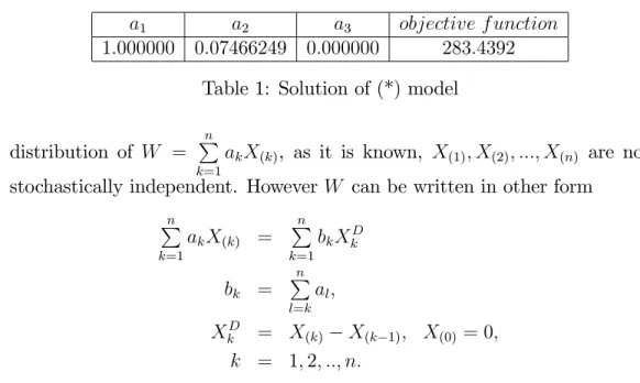
1+ 1:702a1a2 + a22+ 1:448a1a3+ 1:702a2a3+ a23 can be obtained. According to this, with its deterministic equivalent, the problem is max = (3a1+ 2a2+ 1a3)90 1:64485 q (k1a21+ k2a1a2 + k1a22+ k3a1a3+ k2a2a3+ k1a23) 10 (*) k1 32:63246 = 0 k2 55:54045 = 0 k3 47:26492 = 0 0 aj 1 ,j = 1; 2; 3
changed. We can get the solution by using Lingo 9.0 program as below 3.2. Case 2: Order Statistics from the Exponential Population (Dependent Case)
Let X1; X2; :::; Xn be a random sample from F (x) distribution and X(1) X(2) ::: X(n) denote order statistics of this sample. It is interested in
a1 a2 a3 objective f unction 1:000000 0:07466249 0:000000 283:4392
Table 1: Solution of (*) model
distribution of W = n P k=1
akX(k), as it is known, X(1); X(2); :::; X(n) are not stochastically independent. However W can be written in other form
n P k=1 akX(k) = n P k=1 bkXkD bk = n P l=k al; XkD = X(k) X(k 1); X(0) = 0; k = 1; 2; ::; n:
Consequently if the order statistics are taken from the exponential distrib-ution then XD
k ’s have valuable property that is independency. We can use this property for the purpose of work.
Lemma 1 Consider F (x) = 1 e x ; x > 0 and > 0; exponential distribu-tion, then XkD = X(k) X(k 1); with X(0) = 0; k = 1; 2; ::n, are independent. Proof It is su¢ cient to show P X1D > v1; :::; XnD > vn =
n Q k=1
P XkD > vk : Therefore, …rstly it must be found marginal distribution of XD
k . Joint density function of the pair X(r); X(s) , r < s
fX(r);X(s)(x; y) = CF (x)
r 1[F (y) F (x)]s r 1
[1 F (y)]n sf (x)f (y);(4)
C = n!
(r 1)!(s r 1)!(n s)! ; x < y
can be given (see Gibbons, 1971, pp. 29). Hence the common d.f of (X(k 1); X(k)) can be written as follow by assisting (4).
f X(k 1);X(k)(x; y) = n! (k 2)!(n k)! 1 e x k 2 e y n k 2e x y ; x < y From now on, XA
k = X(k 1) auxiliary variable can be de…ned to …nd density function of XkD = X(k) X(k 1):Joint d.f. of XkD; X
A
using the method of Jacobians, f XD k;XAk (vk; x) = C2 1 e x k 2 e (vk+x) n k 2e x e (vk+x) ; x > 0; vk > 0 where C2 = n! (k 2)!(n k)! and the marginal d.f. of XD
k is as follows: (5) f XD k (vk) = e vk (n k+1) C2 1 R 0 1 e x k 2 e x n k+1 e x dx By making e x = transformation, (5) is written in the following form
(6) f XD k (vk) = e vk (n k+1) C2 1 R 0 [1 ]k 2 n k+1d The integral in (6) indicates Beta Function, evaluated as
1 R 0 [1 ]k 2 n k+1d = B (k 1; n k + 2) = (k 2)!(n k + 1)! n! and if it is re written in (6), (7) f XD k (vk) = (n k + 1) e vk (n k+1) vk > 0
is achieved. As it can be seen in (7), XkD has exponential distribution with the parameter (n k + 1) : Now we can …nd joint distribution of random vector XD
1 ; X2D; :::; XnD , on the basis of probability theory
P X(1) > v1; :::; X(n) X(n 1) > vn = n!P (X1 > v1; :::; Xn Xn 1> vn) = n! 1 R v1 1 R v1+v2 ::: 1 R vn+vn 1 ne n P k=1 vk dvn dv2dv1 = n Q k=1 e vk (n k+1)
then the equality is satis…ed. As XD
1 ; X2D; :::; XnD are independent random variables and distributed expo-nential, distribution of W =
n P k=1
bkXkD can be obtained by using convolution technique. We will …rst introduce a de…nition of convolution.
De…nition 1 (Convolution of two functions) The convolution of f and g is written f g. It is de…ned as the integral of the product of the two functions after one is reversed and shifted. As such, it is a particular kind of integral transformation:
(f g)(t) = Z
f (t z)g(z)dz
If X and Y are two independent random variables with probability distri-butions F and G, respectively, then the probability distribution of the sum X + Y is given by the convolution F G:
(8) P (X + Y t) = Z F (t y)dG(y): The distribution of n P k=1
bkXkD can be obtained by iterating (8) as follows
(9) P b1X1D+ b2X2D t = FX1 FX2(t) = t b2 Z 0 FX1( t b2v2 b1 )dFX2(v2) P b1X1D + b2X2D+ b3X3D t = (FX1 FX2) FX3(t) = t b3 Z 0 FX1 FX2(t b3v3)dFX3(v3) .. . P n P k=1 bkXkD t = FX1 FX2 FX3 : : : FXn(t) = t bn Z 0 FX1 : : : FXn 1(t bnvn)dFXn(vn) = 1 n X j=1 Aje thj; where Aj = n Q i=1 i6=j hi hi hj; hj = j bj;and j = (n j + 1) : Hence, P n P k=1 akX(k) t
(10) 1 n X j=1 Aje t(hj) Aj n Q i=1 i6=j hi hi hj = 0; hj (n j+1)bj = 0; bj n P k=j ak = 0 j = 1; 2; :::; n Corollary 1 Let XD k Exp ((n k + 1) ) and FXD k (vk) = 1 e vk(n k+1)
then there exists a stochastic ordering among them as XD
1 st X2D st ::: st XnD:
Proof Firstly de…nition of stochastic ordering may be given; for all t 2 [0;1) ; if P (Y > t) P (X > t) then it is said that X is stochastically less than Y , denoted by X st Y (Shaked and Shanthikumar, 1994, pp. 3). Along with this, for the non negative random variables, recalling the fact that E [X] = 1 R 0 P (X > t) dt; then E [X] E [Y ] , X st Y; relation is obvious. Hence, as E XD k = 1
(n k+1) , the result is satis…ed.
As a result of corollary, if the objective function has the simple special form such as max =
n P k=1
bk then the PCP has the solutions which are expected b1 that is the greatest one and bn that is the smallest one.
Now, deterministic equivalent can be found with another method based on limiting the distribution. This method is called as the …rst edgeworh series expansion and denoted as FE. For further discussion, results are compared with exact distribution method mentioned above.
Theorem 1 Let X1; X2; :::; Xn be independent and continuous random vari-ables such that E jXjj
3
<1 (j = 1; 2; :::; n) , for large values of n,
(11) P 0 B B B B @ n P j=1 Xj E " n P j=1 Xj # q (n) 2 x 1 C C C C A = (x) + (n) 3 (1 x2) 6 (n)2 3 2 (x) + o( n (n) 2 3 2 )
is used approximation to standard normal distribution (Feller, 1966 chapter XVI). Where and stand for standard normal density function, and its distribution function respectively. Here (n)k , k = 2; 3 denotes k. central moment of X: (11) is called …rst term edgeworth expansion in literature (Kendall, 1945, Wallece,1958).
3.3. Set-up for weighted Exponential variates Consider XD
k distributed as EXP ((n k + 1) ), then E XkD = 1 (n k+1) . Hence, the second and third central moments can be obtained as (1)2 =
1
(n k+1)2 2 and
(1) 3 =
2
(n k+1)3 3. From now on, we can reformulate (11), let
M1 = n P k=1 bk(n k+1)1 ; M2 = n P k=1 b2 k(n k+1)1 2 2; M3 = n P k=1 b3 k(n k+1)2 3 3
M1 denotes expectation of weighted sum of n P k=1
bkXkD and M2 denotes sec-ond central moment of
n P k=1
bkXkD and M3 stands for third central moment of n P k=1 bkXkD then P n P k=1 bkXkD t approximated as (12) (x) + M3(1 x2) 6(M2) 3 2 (x); where x = t M1 p M2 By using this expansion, equivalent deterministic constraints of
P n P k=1
akX(k) t can be given as follows
(13) (x) + M3(1 x2) 6(M2) 3 2 1 p 2 e 1 2x 2 M1 n P k=1 bk(n k+1)1 = 0; M2 n P k=1 b2 k 1 (n k+1)2 2 = 0; M3 n P k=1 b3k(n k+1)2 3 3 = 0; x t Mp 1 M2 = 0; bj n P k=j ak = 0; j = 1; 2; ::n
Example 2 Assume that X1; X2; X3 be independent random variables and distributed EXP (0:1) then the problem containing one probabilistic con-straint is de…ned below:
(**) max = a1+a2+a3
P a1X(1)+ a2X(2)+ a3X(3) 15 0:95 a1; a2; a3 > 0 a1; a2; a3 < 1
Solutions are obtained for both method in (10) and (13) which are named as "exact distribution", ED and FE respectively.
Methods a1 a2 a3 objective f unction
ED 0:9999 0:3103 0:0001 1:3103 F E 0:9999 0:2349 0:0001 1:2349 Table 2: ED and FE Solutions of (**) model
As it can be seen from Table2, even if for small values of n FE method’s solution is close to ED.
In the next subsection, we will discuss on the FE method, if the exact dis-tribution of weighted sum can not obtained directly or can not be applicable for PCP. In this situation FE can be more useful to get admissible solution.
3.4. Case 3 Independent and Identically Distributed
Solving PCP by using FE method is considered, if the ED can not give any solution or be applied any more. Let X1; X2; :::; Xn be independent and identically distributed as Rayleigh Distribution, F (x) = 1 e x22 ; x >
0. Consider non negative weights ak and the weighted sum is de…ned as n
P k=1
akXk, then the quantity of P n P k=1 akXk t is related to distribution of n P k=1
akXk. But it is so complicated for some application areas such as PCP that we can o¤er normal approximation called as FE introduced in Theorem1. The expectation, second and third central moments of Rayleigh distribution are given as follows:
= R1 0 xxe x22 dx = r 2 2 = E [X ] 2 = 4 2 3 = E [X ] 3 = r 2( 3) Hence M1 = n P k=1 ak = r 2 n P k=1 ak M2 = n P k=1 a2k 2 = 4 2 n P k=1 a2k M3 = n P k=1 a3k 3 = r 2 ( 3) n P k=1 a3k we can write equivalent deterministic constraints of
P n P k=1 akXk t as follows
(14) (x) + M3(1 x2) 6(M2) 3 2 1 p 2 e 1 2x 2 M1 p 2 n P k=1 ak= 0; M2 42 n P k=1 a2 k= 0; M3 p 2 ( 3) n P k=1 a3k = 0; x t Mp 1 M2 = 0
For two components, exact distribution can be obtained but for more than two components it is hard to …nd it. So that, we …rst give the exact distri-bution for two components, and it can be changed to suitable form to …nd deterministic equivalent of chance constraint.
P (a1X1 + a2X2 t) = t a2 R 0 FX1( t a2x2 a1 )fX2(x2)dx2 = t a2 R 0 1 e 12( t a2x2 a1 ) 2 x2e 1 2x 2 2dx 2 = 1 t a2 p 2 2 pt c a2 1 c a2 a1 t p c a1 a2 t p c 2 pt c a1a2t c3=2 a1 a2 t p c a2 a1 t p c ; c = a 2 1+ a 2 2 We can also give another normal approximation denotes NA as the third method. The following is the deterministic equivalent of (1)
(15) t Mp 1 M2 1( ) M1 p 2 n P k=1 ak = 0 M2 42 n P k=1 a2 k = 0
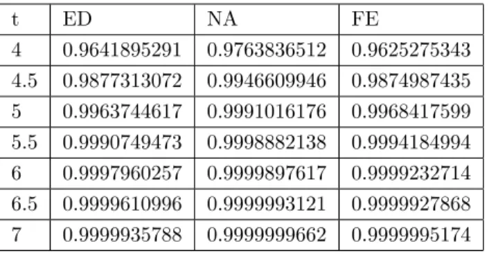
In table3, we have compared our results with the exact distribution for the computed quantity of 1:2X1+:6X2 for some values of t. and tabulated below. But for more than two components the exact distribution is quite complex.
Graphical representation can be given with computed probabilities of 1:2X1+ :6X2 for three methods quantity in …gure1.
Figure 1. Graphs of ED, NA and FE
t ED NA FE .5 0.0046123477 0.0228701744 0.0091353169 1 0.0580212221 0.0765127592 0.0638341739 2 0.4206153212 0.3854435399 0.4150747625 2.5 0.6373180008 0.6093559624 0.6393527753 3 0.8050674871 0.8013620709 0.8080535255 3.5 0.9099386340 0.9215173479 0.9090706369
t ED NA FE 4 0.9641895291 0.9763836512 0.9625275343 4.5 0.9877313072 0.9946609946 0.9874987435 5 0.9963744617 0.9991016176 0.9968417599 5.5 0.9990749473 0.9998882138 0.9994184994 6 0.9997960257 0.9999897617 0.9999232714 6.5 0.9999610996 0.9999993121 0.9999927868 7 0.9999935788 0.9999999662 0.9999995174
Table 4: Computed Probability for 1.2X1+.6X2 (continued)
It can be seen from table3, table4 and …gure1 FE is closer to ED than NA. Example 3
(***) max = a1+ a2
P (a1X1+ a2X2 10) :95 a1 1; a2 1
solution of the problem is obtained by three methods and tabulated below.
M ethods a1 a2 objective f unction N A 2:481026 2:481027 4:962053 F E 2:401541 2:401542 4:803083 ED 2:411933 2:411932 4:823865
Table 5: Solutions of the model (***)
if the objective function is replaced by max = 3a1 + 2a2 with the same constraint, then solution is as given in table6.
M ethods a1 a2 objective f unction N A 3:69094 1:00000 13:07282 F E 3:49001 1:00490 12:47983 ED 3:33075 1:29002 12:57229 Table 6: Solutions of the model for three methods
Even if number of components is small, for both objective functions, FE solutions are close to ED solutions.
4. Conclusion
FE is a limit distribution and for large values of n, it can be close to exact distribution. But we can see that it can be applicable for small values of n. It is possible to use one of two methods, i.e., FE or NA approximations, for two components. As distribution of weighted sum can not be obtained easily, or it may be obtained but can not to be approve for PCP. For those reasons, to obtain equivalent deterministic constraint, which is a stage of solving PCP, it is suggested that NA and FE approximations can be used appropriately. References
1. Charnes A. and Cooper W. W. (1959): Chance-constrained programming, Management Sci. 5, 73–79.
2. Feller, W. (1966): An Introduction to Probability Theory and Its Applications, Volume II. (John Wiley and Sons, Inc. New York, London).
3. Enders, W. (2004): Applied Econometric Time Series, Second Ed., (John Wiley and Sons).
4. Kendall, M.G. (1945): The Advanced Theory of Statistics, Volume I. (Charles Gri¢ n Company Limited).
5. Lehmann, E.L. (1999): Elements of Large Sample Theory, (Springer Verlag, New York Inc.).
6. Wallace, D. L. (1958): Asymptotic approximations to distributions, The Annals of Mathematical Statistics, Vol. 29, No. 3, pp. 635-654.
7. Taha, H.A. (1997): Operations Research on Introduction, (Prentice Hall, Inc. Upper Saddle River, NJ).
8. Gibbons, J.D. (1971): Nonparametric Statistical Inference (McGraw-Hill Book Company).