Solving equations in the universe of hypersets

■ P 3 S

/ 3 3 3

S O L V i r - I G E Q U A T i O N S I f ' i T H

U N I V E R S E O r K Y P E f t S E I S

-i-» ■» Sii V ii· i {«

* A%·* . ^ f: “·.' ;'· > ;■ .'1_{·*·/. .*· V ‘ ‘‘ i}

1 V j .i 'u 3 A ? ^ D ^ V i / - U 'V ·>**■ ·(., .» « V · !» * ' « i Ui : ,i·· ■ V '!■··*'■.

i· « ' i* ‘¿i'rs 6 F -li’ i •1’^^ 1 V. ' A y *ii S .'^ v* *■ 4 4 '‘i ‘ u w Mi i 4t

I'TA \ ■■'**^ri·, ,'*,'> f^ '.;*·· .'•■•A >'W

•t . -I't/ »

'■ w ' u '»•s ^ i : » A U .:.*4 ; T M a : i t V

\ >'i ’''“J .i' V _{• :·; V'. ;· vV.iY .* .,V‘ ;· V .« **•4 d T, T ·'·**'} <-· -·■ * >, ^ i <i_jj »4 s.;s i '¿i TH£ Tw y ... U HI k V J, Xta ^ ·* .SM>;iaMr W i n A ^ V :**■* iiy MuldbZ PAKiCAN i ‘-4 ·*·*''■'·}. i y jf i! CV U 1^'

SOLVING EQUATIONS IN THE

UNIVERSE OF HYPERSETS

A THESIS

SUBMITTED TO THE DEPARTMENT OF COMPUTER ENGINEERING AND INFORMATION SCIENCE AND THE INSTITUTE OF ENGINEERING AND SCIENCE

OF BILKENT UNIVERSITY

IN PARTIAL FULFILLMENT OF THE REQUIREMENTS FOR THE DEGREE OF

MASTER OF SCIENCE

By

Miijdat Pakkaii

February, 1993

РЗ.5

1332

I certify that I have read this thesis and that in my opinion it is fully adequate, in scope and in quality, as a thesis for the degree of Master of Science.

Assoc. Prof. Varol Akman (Advisor)

I certify that I have read this thesis and that in my opinion it is fully adequate, in scope and in quality, as a thesis for the degree of Master of Science.

Prof. Teo Griinberg

I certify that I have read this thesis and that in my opinion it is fully adequate, in scope and in quality, as a thesis for the degree of Master of Science.

in

I certify that I have read this thesis and that in my opinion it is fully adequate, in scope and in quality, as a thesis for the degree of Master of Science.

Asst. Prof. Ilyas Çiçekli

I certify that I have read this thesis and that in my opinion it is fully adequate, in scope and in quality, as a thesis for the degree of Master of Science.

iP-rof. Sinan Serte

Approved for the Institute of Engineering and Science:

Prof. Mehmet ]^ -a y Director of the Institute

ABSTRACT

SOLVING EQUATIONS IN THE UNIVERSE OF

HYPERSETS

Müjdat Pakkan

M.S. in Computer Engineering and Information Science

Advisor: Assoc. Prof. Varol Akman

February, 1993

Hyperset Theory (a.k.a. ZFC ~/A FA ) of Peter Aczel is an enrichment of the classical ZFC set theory and uses a graphical representation for sets. By al­ lowing non-well-founded sets, the theory provides an appropriate framework for modeling various phenomena involving circularity. Z F C /A F A has an im­ portant consequence that guarantees a solution to a set of equations in the universe of hypersets, viz. the Solution Lemma. This lemma asserts that a system of equations defined in the universe of hypersets has a unique solu­ tion, and has applications in areas like artificial intelligence, database theory, and situation theory. In this thesis, a program called HYPERSOLVER, which can solve systems of equations to which the Solution Lemma is applicable and which has built-in procedures to display the graphs depicting the solutions, is presented.

Keywords: Set Theory, ZFC, Non-well-founded Sets, Hyperset Theory (ZFC “ /A F A ), Solving Equations, The Solution Lemma

ÖZET

HİPERKÜMELER EVRENİNDE DENKLEM ÇÖZME

Müjdat Pakkan

Bilgisayar ve Enformatik Mühendisliği, Yüksek Lisans

Danışman: Doç. Dr. Varol Akman

Şubat 1993

Peter Aczel’in (ZFC~/AF.A diye de bilinen) Hiperkûme Kuramı, klasik ZFC küme kuramının zenginleştirilmesiyle ortaya çıkmış ve kümeleri göstermek için çizgeler kullanan bir kuramdır. lyi-yapılanmamış kümeleri de içeren bu ku­ ram döngüsel birçok kavramın modellenmesi için uygun bir ortam yaratır. ZFC “ /A F A kuramının Çözüm Teoremi olarak adlandırılan ve hiperkümeler evrenindeki denklem dizgelerinin çözülebilmesini sağlayan bir sonucu vardır. Bu teorem, hiperkümeler evreninde tanımlanmış bir denklem sisteminin tek bir çözümü olduğunu söyler, ve yapay zeka, veritabanı kuramı ve durum kuramı gibi alanlarda uygulama bulur. Bu tezde. Çözüm Teoremi’nin uygulanabileceği türde denklem dizgelerini çözebilen ve çözümleri çizgeler şeklinde gösterebilen HYPERSOLVER adlı bir program tanıtılmaktadır.

Anahtar Sözcükler: Küme Kuramı, ZFC, lyi-yapılanmamış Kümeler, Hiperkü- me Kuramı (ZFC~/AF.A), Denklem Çözme, Çözüm Teoremi

ACKNOWLEDGMENTS

I would like to thank my advisor Assoc. Prof. Varol Akman who has provided a stimulating research environment and motivating support during my M.S. study. (N.B. Akman’s research has been supported in part by the Turkish Scientific and Technical Research Council, grant no. TBAG -992. Akman thanks Prof. Patrick Suppes, Stanford University, for his generosity in locating some of the references.)

I would also like to thank Prof. Teo Griinberg, Prof. Ahmet Inam, Asst. Prof. Ilyas Çiçekli, and Asst. Prof. Sinan Sertöz for their valuable comments on this thesis.

Finally, I would like to thank everybody who has in some way contributed to rny being myself.

Contents

1 INTRODUCTION

1

2 HYPERSET THEORY

6

2.1 The Anti-Foundation Axiom ( A F A ) ... 6

2.2 The Consistency of the Hyperset T h e o r y ... 10

2.3 Hypersets as a New P a ra d ig m ... 11

3 SOLVING SYSTEMS OF HYPERSET EQUATIONS

15

3.2 A p p lica tion s... 18

3.2.1 Situation T h e o r y ... 20

3.2.2 S t r e a m s ... 21

3.2.3 Relational D a ta b a ses... 22

3.2.4 Modeling Partial In fo r m a tio n ... 24

4 HYPERSOLVER: THE IMPLEMENTATION

25

CONTENTS viii 4.2 Implementation D etails... 31 4.2.1 The User I n t e r fa c e ... 31 4.2.2 In p u t/O u tp u t... 33 4.2.3 Solving E quations... 34 4.2.4 Displaying G r a p h s ... 35 4.2.5 Other F a c ilitie s ... 37

4.3 Limitations and Future W o r k ... 38

5

CONCLUSION

41

A AXIOMS OF ZFC

42

List of Figures

1.1 The cumulative hierarchy starting with 0 and extending to infinity 2 1.2 The one-to-one order preserving cardinality function of Zadrozny 3 1.3 Is the organization of all non-profit organizations (NPO) a mem­

ber of it s e lf? ... 4

2.1 The graph representation of a = {6, {c, d } } ... 7

2.2 The picture of the non-well-founded set = { f l } ... 8

2.3 Unfolding ft to obtain an infinite t r e e ... 9

2.4 Other graphs depicting ... 10

2.5 The relationship between the universes of ZFC and Hyperset T h e o r y ... 12

2.6 The Aczel picture of the proposition p = “This proposition is not expressible in eight words” ... 13

3.1 The solution of the system x = {y, z}, y = {^y}, 2: = {zr;, a:}, tn = 0 16 3.2 The solution of the system x = {C ,j/}, y = { C ,2}, z = . 19 3.3 A relational database consisting of three binary relations . . . . 23

3.4 The SizeOf relation defined for the database in Figure 3.3 . . . . 23

LIST OF FIGURES

4.1 The block diagram of H Y P E R SO L V E R ... 26 4.2 The graph of the stream Z = (A, (B, (C, (D, (E, (F, Z ))}))) . . . . 2S 4..3 An example output of H Y P E R S O L V E R ... 30 4.4 The Command Interface of H YPERSO LVER... 32 4.5 The object class hierarchy of the user interface of HYPERSOLVER 33 4.6 The HYPERSOLVER graph of Q ... 36 4.7 The graphs depicting the solution of the example in Section 4.1 37 4.8 The graphs of the input equations of the example in Section 4.1 37 4.9 The graph of a circular situation S = { R . P , S )... 39

Chapter 1

INTRODUCTION

Set theory has long occupied a unique place in mathematics since it allows var­ ious other branches of mathematics to be formally defined within it [40, 21]. The theory has ignited many debates on its nature and a number of differ­ ent axiomatizations were developed to formalize its underlying ‘philosophical’ principles. Collecting entities into an abstraction for further thought (i.e., set construction) is an important process in philosophy and mathematics, and this brings in assorted problems. The theory had many groundshaking crises (like the discovery of the Russell’s Paradox [19]) throughout its history, which were nevertheless overcome bv various new axiomatizations.

The most popular of these is the Zermelo-Fraenkel axiomatization with ‘ Choice’ (ZFC). ZFC is an elegant theory which inhabits a stable place among other axiomatizations as the mainstream set theory. This is the set theory that is normally taught in basic courses [41]. ZFC has nine axioms (listed in Appendix A) and provides a ‘ hierarchical’ framework. This hierarchy starts with only one abstract entity, the empty set (0), forms sets out of previously formed entities cumulatively, and is therefore called the cumulative hierar­ chy (Figure 1.1). The coherence o f this hierarchy is secured by the Axiom of Foundation (FA) which forbids infinite descending sequences of sets under the membership relation €, such as . . , € C2 G Ui € flo G (thereby not allow­

ing sets which can be constituents o f themselves), and which has sometimes been regarded as a somewhat supexficial limitation [19]. FA states that any nonempty collection A of sets has a member a € A which is disjoint from A

CHAPTER 1. INTRODUCTION

Figure 1.1. The cumulative hierarchy starting with 0 and extending to infinity

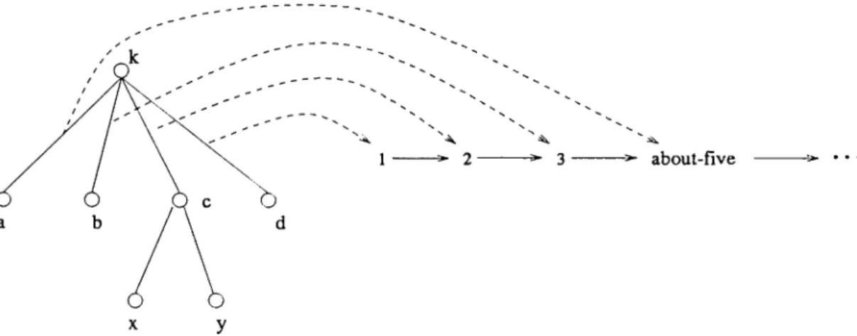
The cumulative hierarchy has provided a precise framework for the formal­ ization of many mathematical concepts [6]. However, it may be asked whether the hierarchy is limiting, in the sense that it might be omitting some interesting sets and concepts one would like to have around [38]. For example, Zadrozny proposes a method of talking about sets which permits (unlike ZFC) some sets to be well-ordered without having an exact cardinality, and vice versa— to have sets with known number of elements which do not necessarily form a well-ordering [49]. For this purpose, leaving the classical notion of cardinality (a one-to-one function from a natural number n onto a set, i.e., a function from a number onto the nodes of the graph of a set) aside, he defines the cardinality function as a one-to-one order preserving mapping from the edges of the graph of a set s into the numerals Nums (an ordered collection of constants denot­ ing numerals and which is linked with sets by existence of a counting routine, denoted by # , and which can take values like 1,2 ,3 ,4 , or 1,2,3, about-five, or 1,2,3, m any). The last element o f the range of # is the cardinality. In this scheme, the representation oi k = {a , 6, { x ,y } ,d } is shown in Figure 1.2. The cardinality of this set is about-five, i.e., the last element of Nums.

ZFC has other drawbacks mentioned in [6]. Besides being too weak to decide some questions like the Continuum Hypothesis, this theory is also too strong in some ways. First, important differences on the nature of the sets are lost in ZFC. For example, being a prime number between 6 and 12 is a different property than being a solution to — 18x 4- 77 = 0, but this differ­ ence disappears in ZFC. Similarly, for an arbitrary Abelian group (G,-t-), the following subgroups of G are not ‘discriminated’ by ZFC while the definitions

CHAPTER 1. INTRODUCTION

about-five

Figure 1.2. The one-to-one order preserving cardinality function of Zadrozny

are increasing in logical complexity:

• pG = {px : X ^ G } = the left coset of (j (p is a fixed element of G)

• T = {x : na; = 0 for some natural n > 0} = the torsion subgroup of G

• \J{H : H is a, divisible subgroup of G] = the divisible part of G

Moreover, a desirable property, the Principle of Parsimony, which states that simple facts should have simple proofs, is quite often violated in ZFC [6]. For example, the verification of a trivial fact like the existence of a x 6 in ZFC relies on the Power Set Axiom [40]. Finally, it can be claimed that mathematical practice suffers from the fact that all the mathematical objects are represented as sets in ZFC. For example, while one can construct in ZFC something iso­ morphic to the real line, the practicing mathematician is not very interested in this [6]. Representing reals as sets could be considered important from a theoretical viewpoint, but one should hardly ever worry about the fact that

\/2 can be determined by the infinite sequence (1,2), (1.4,1.5), (1 .4 1 ,1 .4 2 )....

Cyclic sets, i.e., sets which can be members of themselves, are examples of

interesting sets which are excluded in ZFC. A set like a = {a } is strictly banned in ZFC by the FA since a has no member disjoint from itself. Such sets have infinite descending membership sequences and are called non-well-founded sets.

CHAPTER 1. INTRODUCTION

NPO 6 NPO

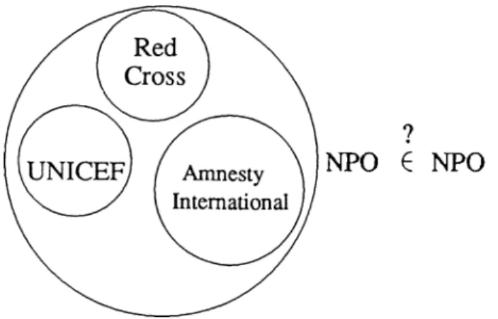
Figure 1.3. Is the organization of all non-profit organizations (NPO) a member of itself?

for a historical review. Non-well-founded sets have generally been neglected by the practicing mathematician ( ‘ the mathematician in the street’ [7]) since the classical well-founded universe was a satisfying domain for his practical concerns. Plowever, non-well-founded sets are useful in modeling various phe­ nomena in computer science, in particular, concurrency, databases, artificial intelligence (A I), etc.

From the standpoint of AI, non-well-founded sets have important applica­ tions. (McCarthy especially stressed the feasibility of using set theory in AI and invited researchers to concentrate on the subject in a 1985 speech [28]. For a recent computational study of set theory that may be relevant to AI the reader is referred to [17].) Circularity is an often exploited property in various fields of AI, e.g., commonsense reasoning. Rehearsing an example by Perils [36], if non-profit organizations are considered as individuals, then the orga­ nization of all non-profit organizations is a set (Figure 1.3). It is conceivable that this umbrella organization (called NPO) might want to be a member of itself in order to benefit from having the status of a non-profit organization (e.g., tax exemption). But this implies that NPO must be non-well-founded, i.e., NPO e NPO.

The importance of circularity in commonsense reasoning has also been men­ tioned in [31, 2, 5, 32]. Circularity is crucial in the representation of meta­ knowledge. In [18, 35], a method which reifies a well-formed formula into a name for that formula (asserting that the name has strong relationship with

CHAPTER 1. INTRODUCTION

the formula) is presented. In this way, any set of well-formed formulas are matched with a set of names, thereby allowing self-reference. In [18], Fefer- man emphasizes the need for type-free (admitting instances of self-application) frameworks for semantics.

This thesis investigates the use of an alternative set theory (due to Peter Aczel [1]) allowing non-well-founded sets. In Chapter 2, the theory of ‘hyper­ sets’ (which is an enrichment of the ZFC set theory) is introduced. (The reader is referred to [22] for a concise yet informative review of Hyperset Theory; also cf. [14].) The theory uses a graph representation for sets. It has an axiom, the Anti-Foundation Axiom (AFA), which replaces the FA of ZFC and informally states that every set, well-founded or not, is representable by a unique graph.

In Chapter 3, a useful consequence of Hyperset Theory is introduced. This is a mathematical result, called the Solution Lemma, which asserts that a system of equations (of some specific form) in the universe of hypersets has a unique solution.

In Chapter 4, HYPERSOLVER is presented. This program solves systems of equations of the sort specified by the Solution Lemma. HYPERSOLVER has built-in graphical utilities to display the graphs depicting the input or solution sets.

Chapter 5 contains the conclusions of the thesis. Appendix A lists the axioms of the ZFC set theory. Appendix B briefly explains how to access HYPERSOLVER.

C hapter 2

HYPERSET THEORY

Hyperset Theory is an enrichment of the classical ZFC set theory. It is the collection of all the conventional axioms of ZFC modified to be consistent with the new universe involving atoms, except that the FA is now replaced by the AFA. The sets in this theory are collections of atoms (urelements) or other sets, whose hereditary membership relation can be depicted by graphs. These sets may be well-founded or non-well-founded, i.e., may have an infinite descending membership sequence, in which case they are named hypersets. Recent studies on Hyperset Theory have been reported in [3].

In this chapter, first, the AFA is explained in Section 2.1, detailing the graph representation used in Hyperset Theory. Then, the consistency of the theory is treated in Section 2.2. Finally, in Section 2.3, the new paradigm introduced by the AFA is discussed and some possible uses in AI are reviewed.

2.1

The Anti-Foundation Axiom (AFA)

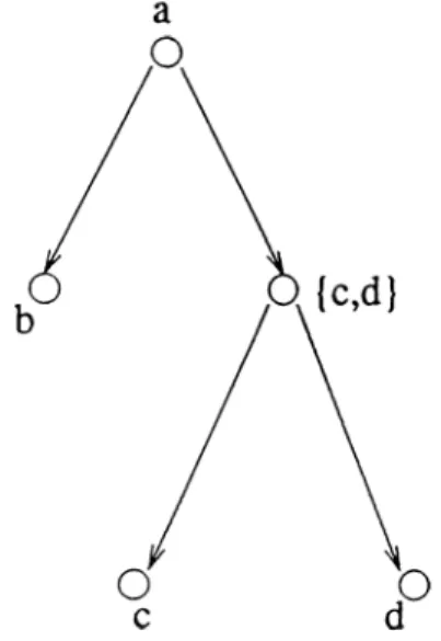
Sets can be pictured by means of directed graphs in an unambiguous manner. For example, a = {6, {c, d }} can be pictured by the graph in Figure 2.1. In this graph, each nonterminal node represents the set which contains the enti­ ties represented by the nodes below it. The edges of the graph stand for the hereditary membership relation such that an edge from a node n to a node m, denoted by n — * m, means that m is a member of n. Since b, c, and d are

CHAPTER 2. HYPERSET THEORY

Figure 2.1. The graph representation of a = {6, {c, cf}}

assumed to contain no other entities as elements (i.e., they are urelements), there are no nodes below them.

To be consistent, Aczel’s terminology will be followed [1]. A pointed graph

is a directed graph with a specific node called its point. A pointed graph is said to be accessible if for every node n, there exists a path no — > ni — > · · ■ — y n

from the point no to n. If this path is always unique, then the pointed graph is a tree and the point is its root. Accessible pointed graphs (apgs) will be used to ‘picture’ sets.

A decoration D for a graph is an assignment of a set to each node of the

graph in such a way that

D(n) = an atom or 0, if n has no children,

{D{77i) : n — > m), otherwise.

An apg G with point n is a picture of the set a if there exists a decoration

D{n) = a, i.e., if a is the set that decorates the top node.

An apg is called well-founded if is has no infinite paths or cycles. Mostowski's

Collapsing Lemma [26] tells us that every well-founded graph has a unique dec­

CHAPTER 2. HYPERSET THEORY

Q

Figure 2.2. The picture of the non-well-founded set i) = { f i }

a unique well-founded set. A non-well-founded apg can never picture a well- founded set because if a is the set which contains all the sets pictured by the nodes occurring in a cycle of the non-well-founded apg, then it can be seen that no member of a is disjoint from a itself, violating the FA.

A czel’s Anti-Foundation Axiom (AFA) states that every apg, well-founded or not, pictures a unique set, or stated in other words, every apg has a unique decoration [1]. AFA has two implications: existence and uniqueness. The former assures that every apg has a decoration (which leads to the existence of non-well-founded sets besides well-founded ones) and the latter asserts that no apg has more than one decoration. By throwing away the FA from the ZFC (and naming the resulting system ZFC“ ) and adding the AFA we obtain the

Hyperset T/ieorj/(a.k.a. ZFC“ /A F A ).

One of the important advantages of the new theory is that by allowing arbitrary graphs, non-well-founded sets are also included. For example, the non-well-founded set Pi = {i7} is pictured by the apg in Figure 2.2, and by the uniqueness property of the AFA, this is the only set pictured by that graph. Therefore, there is a unique set which is equal to its own singleton in the universe of hypersets.

The picture of a set can be unfolded into a tree picture of the same set. The tree whose nodes are the finite paths of the apg which start from the point of the apg, whose edges are pairs o f paths (no — > · · · — > n , uq — > · ■ ■— > n — »· n '), and whose root is the path no of length one is called the unfolding

of that apg. The unfolding of an apg always pictures any set pictured by that apg. Unfolding the apg in Figure 2.2 results in the infinite tree in Figure 2.3,

CHAPTER 2. HYPERSET THEORY O Q u O Q V 0 £ i

Figure 2.3. Unfolding Cl to obtain an infinite tree

analogous to unfolding Cl = { i i } to f2 = { { { · · · } } } · (N.B. Clearly, the right- hand side of the last equality is rather meaningless since the ellipsis does not denote anything.)

The uniqueness property of AFA leads to an intriguing concept of exten- sionality for hypersets. The classical extensionality paradigm, that sets are equal if and only if they have the same members, works fine with well-founded sets. However, this is not of use in deciding the equality of say, a = { l , a } and 6 = {1 ,6 } [12]. The classical extensionality a.xiom is ineffectual here because it just asserts a = 6 if and only if a = 6. However, in the universe of hypersets,

a is indeed equal to b since they are depicted by the same graph. To see this, consider a graph G and a decoration D assigning a to a node x of G, i.e.,

D {x) = a. Now consider the decoration D' e.xactly the same as D except that

D '(x) = b. D' must also be a decoration for G. But by the uniqueness property

of AF.A, D = D\ so D {x) = D'{x), and therefore a = b.

Aczel develops his own extensionality concept by introducing the notion of bisimulation. A bisimulation between two apg's, G\ with point pi and G2 with point P2, is a relation R C Gi x G2 satisfying the conditions

CHAPTER 2. HYPERSET THEORY 10

Q O

Q

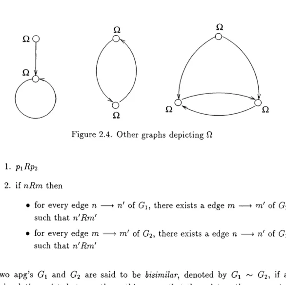
Figure 2.4. Other graphs depicting Q

1. piRp2

2. if nRm then

• for every edge n ■

such that n'Rm '

• for every edge m

such that n'Rm '

n' of G\, there exists a edge m — > m' of G2

m' of G2, there exists a edge n — > n' of G\

Two apg’s G\ and G2 are said to be bisimilar, denoted by Gi ~ G2, if a bisimulation exists between them; this means that they picture the same sets. It can be concluded that a set is completely determined by any graph which pictures it. Therefore, for two sets to be different, there should be a genuine structural difference between them. For instance, the graphs in Figure 2.4 all depict the non-well-founded set = { i f } because their nodes can be decorated with if and there is no essential structural difference between them.

2.2

The Consistency of the Hyperset Theory

The consistency of a theory is related with the absence of paradoxes. In ZFC, the FA was adopted to prevent paradoxes of self-membership. For example, consider the Russell set 2o = (x G a : x ^ x } for any given set a [46]. Russell

had demonstrated that Za ^ a (for otherwise Za G Xa if and only \i za ^ Za).

CHAPTER 2. HYPERSET THEORY 11

is a subset, but not a member of a), and therefore there cannot be a set of all sets. Now let us turn to hypersets to see if Russell’s construction leads to a problem. For a hyperset b = {R i»}, = {1 }. For another hyperset c = {0, { l , c } } , = {0, { l , c } } = c, like all well-founded sets. For neither of these two sets Zx £ x where x = b and x = c, respectively [14]. Therefore, hypersets do not suffer from such constructions.

Showing that Russell’s construction applied to hypersets does not lead to a contradiction does not directly prove that the theory is consistent. Fortunately, Aczel has proved the consistency of the Hyperset Theory by embedding the universe of well-founded sets into the universe of hypersets [1]. For this purpose, he took any domain W of well-founded sets and extended it to get a new domain

V of the universe of hypersets. In this new domain, all the axioms of ZFC~ together with AFA would be true and therefore the consistency of ZFC“ /A F A can be shown. (O f course, this would be relative consistency, relying on the assumption that ZFC“ is consistent.)

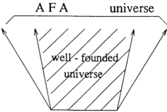
Sets in V are modeled by equivalence classes [G] of apg’s G 6 W, under the bisimulation relation ~ which is an equivalence relation on apgs. Membership relation between these classes is defined as follows: [H] e [G] if and only if there exists a node n which is a child of the top node of G such that ~ G„ where G„ is the sub-apg of G with point n. A set a in F can be represented by the set Ga of the graphs of minimal rank in the cumulative hierarchy which depicts it. Using this construction, it can be shown that all the axioms of ZF C ~ /A F A are true under the above mentioned membership relation and that every well-founded set is uniquely represented in the new universe. Therefore, it can be concluded that the universe of hypersets is a mathematical extension of the universe of well-founded sets. The relationship between them can be depicted as in Figure 2.5.

2.3

Hypersets as a New Paradigm

AFA proposes a new, alternative understanding of set conception. This un­ derstanding may not conform to the classical cumulative conception which has long been the unchanging metaphor of set theory. In this conception, a set is like a box of objects and forming a set is like putting objects in a box. The

CHAPTER 2. HYPERSET THEORY 12

A F A

universe

Figure 2.5. The relationship between the universes of ZFC and Hyperset The­ ory

new conception has also been built on an intuitive rule, viz. structure forgetting

[14]. Taking any structured object with ‘components’ (i.e., any set with ele­ ments), one can forget the components and is left with an abstract set-theoretic structure. The difference between the two metaphors is where these objects come from and what they are. In the classical cumulative picture, starting with 0 (or a set of atoms) any set can be formed, which in turn can be used to form new sets. However, sets formed in this manner will all be well-founded. But in the structure forgetting metaphor, every set, well-founded or not, can be represented as a structured object, namely a directed graph. This has a straightforward analogy with the extension of rational numbers first to real numbers, and then to complex numbers.

AFA has important applications in various fields of computer science. In [12], a modeling scheme for propositions (of natural language) is offered. In this scheme, the triple (P, p, ¿) denotes that the proposition p has the property P if f = 1, and it does not have it if i = 0. (In set theory, triples like { x, y, z)

are defined as pairs of pairs, i.e., ( x, { y, z) ) , and (y,z) ^ {{î/}? {î/>-2^}}·) F the proposition p is taken to be say, the statement

“This proposition is not expressible using eight words,”

then it can be modeled by the triple ( £ ’,p, 0) where E (an atom) is the property of being expressible (in English) using eight words. In Aczel’s conception, p can be depicted as in Figure 2.6 where the longest arc shows that p refers to

CHAPTER 2. HYPERSET THEORY ₁₃

Figure 2.6. The Aczel picture of the proposition p

expressible in eight words”

= “This proposition is not

itself.

Mislove, Moss, and Oles [29] developed a partial set theory ZFAP based on

protosets which is a generalization of HF, the set of well-founded hereditarily

finite sets. A protoset is like a well-founded set except it has some packaging

which can hide some of its elements. There exists a protoset J_ which is empty except for packaging. From a finite collection x i , . . . , x„, one can construct the

clear protoset { x i , . . . , x „ } which has no packaging, and the murky protoset

[ x i ,. . . , x„] which has some elements, but also packaging. For example, a murky set [2,3] contains 2 and 3 as elements, but it might contain other elements, too. By definition, X is clarified by y, x C y, if one can obtain y from x by taking some packaging inside x and replacing this by other protosets.

ZFAP has a first-order language L with three relation symbols: € (for actual membership), €<> (for possible membership), and set (for set existence).

CHAPTER 2. HYPERSET THEORY 14

The theory consists of two axioms (Piet and PSA) and which is the relativization of all axioms of ZFC~/AFA to set. The axiom

(Piet) (V x3G )[sei(G ) A “ G is a partial set graph”

A {3d)(d = D{G) A d(rootc) = x)]

states that every partial set has a picture, viz. a set G which is a partial set

graph (corresponding to an apg in Aczel’s terminology) such that there is a

decoration d of G with the root decorated as x. The axiom

(PSA) (V G )[(sei(G ) A “ G is a partial set graph” ) (3!d)(d = D{G))]

Chapter 3

SOLVING SYSTEMS OF

HYPERSET EQUATIONS

AFA has an important consequence which has useful applications and is the main point of this thesis. This consequence allows us to assert that some sets exist without having to picture them with graphs and will be motivated by the following example [1].

An equation of the form x = (0, x) in one variable x can be rewritten as

X = { { 0 } , {0 ,a :}}. This equation is equivalent to the following system of four equations in four unknowns:

y =

r/; = 0.

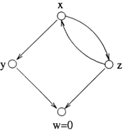
By AFA, this system of equations has a unique solution pictured by the graph in Figure 3.1. Unfolding the original equation, one obtains x = {0, (0, ( 0 ,...) ) ) . This result can be generalized. It can be shown that for any set a, the equation X = (a ,x ) has a unique solution x = (a, {o, ( a ,...) ) ) . More generally, if we consider an infinite system of equations

CHAPTER 3. SOLVING SYSTEMS OF HYPERSET EQUATIONS 16

Figure 3.1. The solution of the system x = { y, z} , y = { w} , z = {tu ,x }, to = 0

Xq — ( ^0_{) ^}1₎₎

X i = ( a i , X2_),

^2 = («2) 3:3),

then a unique solution

Xq = (a o ,(a i,(a2, . . . } } } ,

X i = ( a i , ( 0 2 , ( 0 3 , . . . ) } } , x-2 = ( 0 2 , ( 0 3 , ( 0 4 , . . . } } } ,

is seen to exist.

Motivated by such examples, a technique to assert that every system of equations has a unique solution has been developed by Aczel [1]. This tech­ nique is named the Solution Lemma by Barwise and Etchemendy [12] and is formulated in Section 3.1. Section 3.2 contains some possible applications of the lemma.

CHAPTERS. SOLVING SYSTEMS OF HYPERSET EQUATIONS 17

3.1

The Solution Lemma

Let Va be the universe of hypersets with atoms from a given set A and let

Va' be the universe of hypersets with atoms from another given set A! such that A C A' and X A' — A. The elements of X can be considered as

indeterminates ranging over the universe Va· The sets which can contain atoms

from X in their construction are called X-sets. A system of equations is a set of equations

{x = : X ^ X A Ci is an X -set}

for each x E X . For example, choosing X = { x , y , z } and A = {C ,M } (thus

A = {x , y, X, C, M }), consider the system of equations ^ ~ { C ,y },

2/ =

X = {M , x }.

A solution to a system of equations is a family of pure sets bx (sets which

can have only sets but no atoms as elements), one for each x £ X , such that for each x E X , bx = irax. Here, tt is a substitution operation (defined below) and na is the pure set obtained from a by substituting bx for each occurrence of an atom x in the construction of a.

The Substitution Lemma states that for each family of pure sets bx {x E X ),

there exists a unique operation tt which assigns a pure set na to each X-set a,

viz.

7

7

6

6

The Solution Lemma can now be stated [1]. If is an X-set, then the system

of equations x — ax{ x E X ) has a unique solution, i.e., a unique family of pure sets bx such that for each x E X, = wax.

This lemma can be stated somewhat differently [14]. Letting X again be the set of indeterminates, g a function from X to 2^, and h a function from

X to A, there exists a unique function / for all x G A such that

Obviously, g{x) is the set of indeterminates and h(x) is the set of atoms in each

X-set ttx of an equation x = Ox. In the above example, g{x) = {?/}, g{y) = {z},

g{z) = { x } , and h(x) = { C } , h[y) = {C }, h(z) = {M }, and one can compute

the solution

/ ( x ) = { C , { C , { M , x } } } , / ( j / ) = { C , { M , { C , y } } } , /( ^ ) = { M , { C , { C , z ) } ) . These are depicted in Figure 3.2.

The Solution Lemma is an elegant result, but not every system of equations has a solution. First of all, the equations have to be in the form suitable for the Solution Lemma. For example, a pair equations such as

^ = {2/ ,2},

y =

cannot be solved since it requires the solution to be stated in terms of the indeterminate x. (These are analogous to the Diophantine equations.) As another example, the equation

X = 2^

cannot be solved because Cantor has proved (in ZFC~) that there is no set which contains its own power set (no matter what axioms are added to ZFC” ) [47].

CHAPTER 3. SOLVING SYSTEMS OF HYPERSET EQUATIONS 18

3.2

Applications

This technique of solving equations in the univ'erse of hypersets is an important mathematical result because it allows us to assert the existence of some sets (the solutions of the equations) without having to depict them with graphs. This feature can be of considerable help in modeling information which can be cast in the form of equations. In this section, examples concerning Situation Theory, relational databases, and streams are reviewed.

CHAPTER 3. SOLVING SYSTEMS OF HYPERSET EQUATIONS 19

CHAPTER 3. SOLVING SYSTEMS OF HYPERSET EQ UATIONS 20

3.2.1

Situation Theory

Situation Theory is a theory of meaning and information content developed by

Barwise and Perry [15]. It tries to formalize a semantics for English in the way English speakers handle information.

A situation is a limited portion of the reality. It can be taken as a whole

interacting with other situations. An infon is an ordered list (R,a,i) where i? is a relation, a is an assignment of objects of the real world, and i is the polarity, taking 0 or 1 as its value. For a given R and a, only one of the two infons <7 = {R, a, 0) от a = { R, a, l ) is a fact, namely the one which holds in some situation s. (This is denoted by s |= a.) For example, the infon

{sleeping^ Tom, garden^ 1) is a fact if and only if Tom is indeed sleeping in the

garden. (As a notational convention, a polarity 1 is usually dropped.)

It is generally hypothesized that situations are sets of facts and therefore can be modeled by sets to make use of the existing set-theoretic techniques !3-3. 4]. Indeed, this was the approach Barwise and Etchemendy chose in [15]. However, using Barwise’s Admissible Set Theory [6] as the principal mathematical tool in the beginning led to problems in the handling of circular situations and they had to turn to the Hyperset Theory [10]. To demonstrate this, an example concerning common knowledge will now be given, viz. the Conway paradox [9]. Two card players Pi and P2 are given some cards such that each gets an ace.

Thus, both Pi and P2 know that the following is a fact:

a : Either Pi or P2 has an ace.

When asked whether they knew if the other one had an ace or not, they both would answer ‘no’ . If they are told that at least one of them has an ace and asked the above question again, first they both would answer ‘ no’ . But upon hearing Pi answer ‘no’ , P2 would know that Pi has an ace. Because, if Pi does not know P2 has an ace, having heard that at least one of them does, it can only be because Pi has an ace. Obviously, Pi would reason the same way, too. So, they would conclude that each has an ace. Therefore, being told that at least one of them has an ace must have added some information to the situation. How can being told a fact that each of them already knew increase their information? This is the Conway paradox. The solution relies on the fact that initially the fact cr was know^n by each of them, but it was not common

knowledge. Only after it became common knowledge, it gave more information. Hence, common knowledge can be viewed as iterated knowledge of cr of the following form: Pi knows <7, P2 knows <r, P\ knows P2 knows <7, P2 knows

P\ knows <7, and so on. This iteration can be represented by an infinite se­

quence of facts (where K is the relation ‘ knows’ and s is the situation in which the above game takes place): {K, Pi, s), ( K, P2,s), {K, Pi, {K, P2, s)), { K , P 2 , { K , P i , s } ) , . . .

However, considering the system of equations

x = { { K , P i , y ) , { K , P2, y)}, y = s U { { K , P i , y ) , { K , P2,y)},

the Solution Lemma asserts the existence of the unique sets s' and s U s' s itisfying these equations, respectively, where

s' = { { K , P i , s U s ' ) , { K , P2,s\Js')].

Then, the fact that s is common knowledge can more effectively be represented by s' which contains just two infons and is circular.

3.2.2

Streams

CHAPTER 3. SOLVING SYSTEMS OE HYPERSET EQUATIONS 21

Streams are abstract data structures. A stream is an ordered pair s = {a, s')

where a is an element of a set A o f atoms and s' is another stream. Thus, a stream is a sequence of elements, possibly infinite, e.g.,

(0, (1, (2, . . . ) ) ) .

Streams are largely used for character input/output in functional languages like Lisp [39] and ML [48]. A stream in such a language is an abstract concept which captures the essential properties of a data producer (an existing file, the keyboard, a program, etc.) or a data consumer (the screen, a program, etc.) For example, an input stream is where one gets the input characters which the user enters through a program (the characters become the atoms in this case).

If one wants to model the collection of streams each having an atom from the set A as the first element, then the set S{A) can be defined as the largest

set satisfying the condition: if .s 6 5'(i4), then s = some a E A and s' G Intuitively, every infinite sequence of atoms should lead to a stream. However, assuming the FA, »^(A) = 0 because any such stream gives rise to an infinite descending chain in the membership relation, thus violating the axiom [14].

Nevertheless, in ZFC ~/A FA , it can be shown that every infinite sequence Co, 0 1,0 2, . . . can lead to a stream like (0 0, (0 1, (0 2, . . . ) ) ) , by making use of

the Solution Lemma. To elucidate our point, take the following system of equations:

Xq — (oq,2:i),

Xi — (o i, X2} 1

X 2 — ( 0 2 5 ^ 3 ) 9

The solution to this system,

Xq (oQ) (oi, (0 2, . . ·))))

X i = ( 0 1 , ( 0 2 , ( 0 3 , . . . ) ) ) , X2 (o2) (o3) (0 4, . . ·)))·

includes the desired stream, namely the value of .To· A generalization of this to arbitrary sequences can be found in [1 2].

3.2.3

Relational Databases

CHAPTER 3. SOLVING SYSTEMS OF HYPERSET EQUATIONS 22

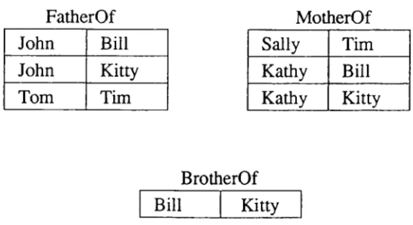
Relational databases embody data in tabular forms and show how certain ob­ jects stand in certain relations to other objects [45]. As an example adapted from [11], the database in Figure 3.3 includes three binary relations: FatherOf, MotherOf, and BrotherOf. Binary relations can be represented as sets of or­ dered pairs such that if an object o stands in relation R to another object

6, denoted by aRb, then (a, b) ^ R. A database model is a function AI with

domain some set Rel of binary relation symbols such that for each relation symbol R € Rel, R^^ is a finite binary relation that holds in model A /.

CHAPTER 3. SOLVING SYSTEMS OF HYPERSET EQUATIONS 23

FatherOf

MotherOf

John

Bill

John

Kitty

Tom

Tim

Sally

Tim

Kathy

Bill

Kathy

Kitty

BrotherOf

Kitty

Figure 3.3. A relational database consisting of three binary relations

SizeOf

FatherOf

3

MotherOf

3

BrotherOf

1

SizeOf

4

Figure 3.4. The SizeOf relation defined for the database in Figure 3.3

If one wants to add a new relation symbol SizeOf to this database, then

Rel' = Rel U {SizeO f}. A database model M for Rel' is correct if the relation

SizeOf^^ contains all pairs {R,n) where R E Rel and n = \R\. (| · | stands for the cardinality function.) Such a relation can be seen in Figure 3.4. Now it may be taken for granted that every database for Rel can be extended in a unique way to a correct database for Rel'. Unfortunately, this is not so.

Assuming the FA, it can be shown that there are no correct database models. Because if M is correct, then the relation SizeOf stands in relation SizeOf to n, denoted by SizeOf SizeOf n. But this is not true in ZFC because otherwise (SizeOf, n) E SizeOf.

If Hyperset Theory is used as the meta-theory instead of ZFC in modeling such databases, then the solution o f the equation

CHAPTER 3. SOLVING SYSTEMS OF HYPERSET EQUATIONS 24

(which can be found by applying the Solution Lemma) is the desired SizeOf relation.

3.2.4

Modeling Partial Information

The technique of solving equations in the universe of hypersets can be exploited to model partial information [8]. For this purpose, the objects of the universe

Va of hypersets over a set A of atoms can be be used to model non-parametric objects, i.e., objects with complete information. The set X of indeterminates can be used to represent parametric objects, i.e., objects with partial informa­ tion. The universe of hypersets on A U X is denoted as analogous to the adjunction of indeterminates in algebra.

For any object a £ the set

par{a) = { x £ X : x G TC{a)} ,

where TC(a) denotes the transitive closure of a, is called the set of parameters of a. If a € Vai then par{a) = 0 since a does not have any parameters. An

anchor is a function / with domain{f) C X and range(f) Q Va — A which

assigns sets to indeterminates. For any a G V.4[A’] and anchor / , a{ f ) is the object obtained by replacing each indeterminate x G par (a) fl domain{f) by the set f { x ) in a. This is accomplished by solving the resulting equations by the Solution Lemma. In this way, the anchoring of parameters is modeled.

Parametric anchors can also be defined as functions from a subset of X

into VyijA’ ] to assign parametric objects, not just sets, to indeterminates. For example, if a(a:) is a parametric object representing partial information about some non-parametric object a E Va and if one does not know the value to which

X is to be anchored, but knows that it is of the form b{y) (another parametric

object), then anchoring x to b{y) results in the object a{b{y)) which does not give the ultimate object perhaps, but is at least more informative about its structure.

Chapter 4

HYPERSOLVER:

THE IMPLEMENTATION

HYPERSOLVER is a stand-alone program which can solve equations in the universe of hypersets by making use of the Solution Lemma. It has built-in graphical capabilities for displaying the graphs depicting the equations input by the user and the solutions of these equations. HYPERSOLVER is implemented in Lucid Common Lisp. To communicate with the user and to display graphs, it makes use of the XView Window Toolkit built on the X Window System.

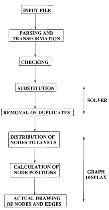
H YPERSOLVER’s block diagram is shown in Figure 4.1 which depicts the main functions. The functionality of the program will be explained in Sec­ tion 4.1. Then, in Section 4.2, implementation details of the user interface, file input/output, equation solving, and graph display will be given. This will be followed by the limitations of HYPERSOLVER and possible future work in Section 4.3.

4.1

Functionality

HYPERSOLVER solves a system of equations in the universe of hypersets. By a system of equations, the definition in Section 3.1 is meant:

{ x = Ox : X E X and Ox is an X-set }

CHAPTER 4. HYPERSOLVER: THE IMPLEMENTATION 26

SOLVER

GRAPH DISPLAY

CHAPTER 4. HYPERSOLVER: THE IMPLEMENTATION 27

for each x X , where X is a set of indeterminates, is a set of atoms, and

an X-set is a set which can contain elements from X . HYPERSOLVER does

not solve systems which are not of this form. Therefore, taking A = { 0 ,1} and

X — { x ,2/} , a system like

{0, l , y } ,

y = {a;},

is a valid input for HYPERSOLVER, while the single equation

or the system

1 = { x ,2/ ,0},

x = {0,1},

X = {x }.

are not since 1 ^ X and there should be a single equation for each x € A’ . (HYPERSOLVER includes some filtering functions to detect invalid input and warn the user.)

The notational conventions in HYPERSOLVER are as follows. Letters A through L are used to represent atoms of A, while letters M through Z represent indeterminates of X . The symbol @ will be used to represent the non-well- founded singleton fl. (One-letter variable naming may seem quite limiting but it is simple to adopt the parser to handle variables with longer names.) Therefore, the graph depicting the stream Z = (A, (B, (C, (D, (E, (F, Z )))))) is output as in Figure 4.2 by HYPERSOLVER, where dummy variables such as M, N, 0 , . . . are assigned to intermediate nodes. These dummy nodes depict the sets which are formed by the children of those nodes, e.g; M = { { B M { C } , { . . . } } } .

HYPERSOLVER gets its input from a file which is to be specified by the user. The file must have one equation per line with no space characters occur­ ring in the equations. For example, a file consisting of the following lines is a valid input file:

X = { X , Y ) , Y = ( A , B , Y , Z } ,

CHAPTER 4. HYPERSOLVER: THE IMPLEMENTATION 28

S HYPERSOLVER

CLICK A MOUSE BUTTON...

CHAPTER 4. HYPERSOLVER: THE IMPLEMENTATION 29

The input read from the file is sent to the parser of HYPERSOLVER. The parser is a character checking parser with a lookup table for the input charac­ ters. After converting the input into Lisp form, a transformation is applied to convert it to a list that can be processed by the equation solver.

The equation solving step of the HYPERSOLVER applies the Solution Lemma to the input system of equations. The alternative formulation men­ tioned in Section 3.1 is used for this purpose:

/ ( ^ ) = { / ( y ) : y e y(a;)} U h{x),

for any set X of indeterminates where ^ is a function from X to 2^ and h is

function from X to a set A of atoms. For the above example set of equations, i ( X ) = { X ,Y ) , i,(Y ) = { Y ,Z ) , g(Z) = { X ,Y } and k{X) = 0, h{Y) = { A ,B } ,

h(Z) = { @ } = @. This representation scheme is suitable for recursive sub­

stitution. The algorithm of the equation solver performs this substitution by applying the Substitution Lemma on each equation of the input equation sys­ tem. So, the solution for an indeterminate X can be found by finding the solutions of the indeterminates in 5'(X) recursively. For each indeterminate,

a decoration is found and the solutions are expressed in terms of these deco­ rations. For example, the decorations of the graphs for the above system of equations are (p, ç, and r are the decorations for the indeterminates X, Y, and Z, respectively):

p={®,{A,B,®,{p,q,Q}}},

q={A,B,®,{{Q,q},q,<

r={{<3,q},{A,B,®,r},(

The next step is the invocation of the graph display part of the H YPER­ SOLVER. This part takes the solution of a system of equations produced by the equation solver as input. As the general graph layout algorithm, a variant of the hierarchical layout algorithm proposed in [37] is exploited. The reason to use a hierarchical layout algorithm instead of a general-purpose algorithm is that most of the equations to be solved by the Solution Lemma will be hi­ erarchical and that self-reference generally occurs for a single indeterminate. (Figure 2.6 is a good example of this.) A hierarchical algorithm leads to sim­ plification in the display procedui'e and efficiency in run time.

CHAPTER 4. HYPERSOLVER: THE IMPLEMENTATION 30

S HYPERSOLVER

Figure 4.3. An example output of HYPERSOLVER

The algorithm which has been adapted to the representation conventions and output requirements of HYPERSOLVER first forms the edge list of the solution system which consists of pairs of nodes. This list helps to get all children of each indeterminate. Then the nodes corresponding to these children are distributed to the levels taking care of the relationships between pairs of nodes. A more complicated part of the graph display unit is the one calculating the positions of the nodes on the screen. The hierarchical nature of the solution graphs is again exploited to make this calculation. The positions of the descendants of a node are calculated with respect to its own position, which in turn has been calculated with respect to its antecedents.

After the calculation of the positions, the actual graph drawing procedure is activated to display first the nodes and later the edges. This procedure pops up a large window (called the Graph Display Window, GDW) on which all graphical information is put. The output convention is such that the node labels which are the decorations o f the sets represented by those nodes are written inside the node boundaries. Intermediate nodes which represent sets as lower-level children are displayexl only by their labels. This can be seen in the first graph of the Figure 4.3 where the node labeled Y is in fact decorated by { C ,Z } . The graphs of the solutions to a system of equations are displayed independently side by side on the GDW. The user can exit this window by pressing any button of the mouse. An example output of HYPERSOLVER is shown in Figure 4.3 where the input equations are taken from Section 3.1.

CHAPTER 4. HYPERSOLVER: THE IMPLEMENTATION 31

4.2

Implementation Details

4.2.1

The User Interface

HYPERSOLVER has been implemented in Lucid Common Lisp [39]. It com­ municates with the user through the XView Window Toolkit [23] based on the X Window System [30]. XView allows a programmer to build user interfaces without having to learn details of the underlying window system, thereby sim­ plifying application development. It is an object-oriented toolkit whose objects constitute the user interface. Examples of these objects are frames, canvases, panels, buttons, etc. These objects are represented in a class hierarchy and may activate other procedures performing various tasks when triggered by an input event.

XView is accessible from within Lucid using the rXVIEW package with a foreign function interface. XView foreign function calls return an address to the object or value they produce. For example, a canvas which is a child of a frame say, fram el (which must have been created before), is created by the following command ( x v -c r e a t e fram el : CANVAS x v -x 0 x v -y 0 x v -w id th 300 x v -h e ig h t 2 0 0)

Here, the first parameter (frcim el) is the parent, the second ( : CANVAS) is the type, the third and the fourth (x v -x and x v -y) are the x and y coordinates, and rest (x v -w id th and x v -h e ig h t) are the width and height of the new object. This command returns an address to the new canvas object. However, the objects created by x v -c r e a t e are not directly displayed on the screen. The XView command x v -m a in -lo o p accomplishes this. Its main task is to call the Notifier of the XView. The Notifier is where the main control loop resides. It receives and processes events such as keyboard or mouse input, window resizing, etc. After reception of an event, an application-specific callback routine can be called to take appropriate action according to the event. A callback routine is

CHAPTER 4. HYPERSOLVER: THE IMPLEMENTATION 32

H Y P E R S O L V E R

FILENAME:

(

)

(

)

OPTIONS

( S E E IN P U T j

(SOLUTION^

(

)

(

)

Figure 4.4. The Command Interface of HYPERSOLVER

a procedure which is previously registered with the Notifier by the application, and is notified, i.e., called out by the Notifier upon some event [23]. After a callback routine ends, control returns back to the Notifier. In Lisp, these callback routines should be defined such that they can be called from the Notifier which is a foreign-function in the C language [25]. Therefore, the callback routines in HYPERSOLVER are defined as

( d e f - f o r e i g n - c a l l a b l e (function name))

As the x v -m a in -lo o p is called, the Command Interface of FIYPERSOLVER shown in Figure 4.4 appears on the screen waiting for user input. This is a panel object with a text input field and six buttons. The object class hierarchy of this interface is depicted in Figure 4.5.

CHAPTER 4. HYPERSOLVER: THE IMPLEMENTATION 33

Figure 4.5. The object class hierarchy of the user interface of HYPERSOLVER

4.2.2

Input/Output

File input/output facilities of HYPERSOLVER consist of loading an input file containing the input equation system and writing the solution of that system to an output file, both of whose names must be specified by the user. Click­ ing the LOAD button of the Command Interface activates the foreign-function callable g e t -in p u t. This function reads the value of the panel text input field and opens the input file whose name is that value. The value can contain a pathname to the file also. Then, the function reads the equations (one equation per line) from that input file. The input is in string form and is converted into a form required by the solver, viz. a list of equations which are themselves lists consisting of the indeterminate x as the head and the X-set as the rest of the list. The example system o f equations in Section 4.1 have the following representation when transformed into this form:

(X X Y), (Y A B Y Z);

CHAPTER 4. HYPERSOLVER: THE IMPLEMENTATION 34

This transformation is performed by p arse-an d-tran sform . This function parses each character in the string by looking for its value in a lookup table which has been implemented using the hash-table feature of Common Lisp [39]. This lookup value is appended to a list and finally this list forms the input equation system.

The input equation system is then checked for validity by check. Currently, this function only checks if there exists one equation for each indeterminate in the system and whether each equation is in the required form x = a^. If it finds an error, check notifies the user and aborts the program.

Clicking the SAVE button activates the foreign-function callable save-outpu t. The task of this function is simply to read the value of the panel text input field and write the solution which has been obtained by solving the input system to the file whose name is specified by that value. Before writing, the solution which is in list form is converted into string form by treaisf orm-output.

4.2.3

Solving Equations

The equation solving unit of HYPERSOLVER is a function which applies the Solution Lemma to each equation in the input system. For this purpose, the Substitution Lemma of Section 3.1 is applied to each equation recursively so that all nested indeterminates are substituted by their corresponding decora­ tions. The solver cannot solve equations to which the lemma is not applicable. The SOLUT I O N button is the main triggering point of the equation solver. Clicking it activates the foreign-function callable s o lv e r which constitutes the main body of the equation solver. It invokes s u b s t it u t e r for each equation in the input equation system. This function is where the substitution implied by the Substitution Lemma is performed. Each indeterminate of the equation is substituted with its value, which is either an atom or another X-set. (If its value is equal to itself, then this denotes self-membership and Q is used to signal that.) In the latter case, a recursive substitution is needed to substitute the values of the indeterminates occurring in that X-set. To prevent duplicate substitutions which arise when an indeterminate occurs two or more times in

CHAPTER 4. HYPERSOLVER: THE IMPLEMENTATION 35

because of the nature of recursion, duplication may occur in different levels of set nesting. Therefore, s o lv e r applies a kind of filtering on the output of s u b s t it u t e r by activating rem ove-du plicates. This last function simply checks the solution list and removes any duplicate substitutions. For example, the solution of the above example equation system (generated by s u b s t it u t e r )

((X 0 (Y A B ® (Z X Y 0))) (Y A B 0 (Z (X 0 Y) Y 0))

(Z (X 0 (Y A B 0 Z)) (Y A B 0 Z) 0))

contains a duplicate substitution of Y in the solution of the indeterminate Z. This duplication is removed as a result of this filtering.

4.2.4

Displaying Graphs

The final task of s o lv e r is to invoke d is p la y -s o lu t io n to display the graphs depicting the solutions by supplying the solution system as the input. This function starts with forming the edge list for every graph depicting an indeter­ minate, by calling form -edges. The output is given to f o r m - c h i l d - l i s t to build the list of the children of every node in the solution. For efficiency pur­ poses, an association list which provides quick access to data is used [39]. Then, nodes are assigned to the levels of the hierarchy by a s s ig n -n o d e s -t o -le v e ls taking care of hereditary membership and neighborhood relations.

The next step is to find the positions of the graphs on the screen. Placement of the graphs on the screen is a difficult problem. HYPERSOLVER does not yet support scrolling facilities. Therefore, careful planning for properly placing the graphs on the screen is needed. For this purpose, the maximum width of each graph in the solution system is calculated by checking the level hierarchy. If the width of the last processed graph exceeds the right boundary of the GDVV, then it is carried to the leftmost side below the previous equations’ graphs. (This is analogous to feeding a CRLF character to a printer.) The function f i n d - p o s i t i o n s calculates the coordinates for each node in the system. It maintains an association list for this purpose, keeping the x, y coordinates, level information, and a flag to indicate self-membership of each node. This function calculates the position of a node with respect to its antecedents. The