Multicriteria inventory classification using a genetic algorithm

(1)

JOURNAL OF OPERATIONAL

RESEARCH E L S E V I E R European Journal of Operational Research 105 (1998) 29-37

T h e o r y a n d M e t h o d o l o g y

Multicriteria inventory classification using a genetic algorithm

H . A l t a y G u v e n i r a'*, E r d a l E r e l b

a Department of Computer Engineering and Information Science, Bilkent University, 06533 Ankara, Turkey b Department of Business Administration, Bilkent University, 06533 Ankara, Turkey

Received 19 August 1996; accepted 4 December 1996

Abstract

One of the application areas of genetic algorithms is parameter optimization. This paper addresses the problem of optimizing a set of parameters that represent the weights of criteria, where the sum of all weights is 1. A chromosome represents the values of the weights, possibly along with some cut-off points. A new crossover operation, called continuous uniform crossover, is proposed, such that it produces valid chromosomes given that the parent chromosomes are valid. The new crossover technique is applied to the problem of multicriteria inventory classification. The results are compared with the classical inventory classification technique using the Analytical Hierarchy Process. @ 1998 Elsevier Science B.V. Keywords: Computers; Genetic algorithms; Analytical Hierarchy Process; Inventory; Multi-criteria analysis

1. Introduction

It is not uncommon to observe companies of even moderate sizes to carry thousands of different items in inventory. These items are kept for various purposes and include raw materials, components used in products, items used for activities to support production such as maintenance, cleaning, etc. Recently, the number of items carried in inventory increased drastically with the increase of customer pressure demanding different models of products. In order to obtain a com- petitive advantage in the market, companies have to respond to satisfy the various demands of customers; this results in an increased number of different items carded in inventory in smaller quantities.

Faced with the heavy burden of dealing with a large number of items, companies must classify the items in inventory and develop effective inventory control poli-

* Corresponding author. E-mail: guvenir@bilkent.edu.tr

cies for these classes. The classical ABC classification, developed at General Electric during the 1950's, is the most popular scheme to classify the items in inventory. The scheme is based on the Pareto principle of the 18th century economist, Villefredo Pareto, stating that 20% of the people controlled 80% of the wealth. Empirical studies indicate that 5-20% of all items account for 55-65% of total dollar volume, 20-30% of all items account for 20-40% of total dollar volume, and the remaining 50-75% of all items account for only 5-25% of total dollar volume. In the classical ABC classification, items are ordered in descending order of their annual dollar usage values which are the products of annual usage quantities and the average unit prices of the items. The relatively small number of items at the top of the list controlling the majority of the total an- num dollar usage constitutes class A and the majority of the items at the bottom of the list controlling a relatively small portion of the total annual dollar usage constitutes class C. Items between the above classes

(2)

30 H.A. Guvenir, E. Erel/European Journal of Operational Research 105 (1998) 29-37

constitute class B. The designation of these classes is arbitrary and the number of classes may be increased depending on the extent to which a firm wants to dif- ferentiate control efforts. Tight management control of ordering procedures and individual demand forecasts should be made for class A items. Class C items should receive a loose control, such as a simple two-bin system, and class B items should have a control effort that lies between these two extremes. Thus, in a typical firm, concentrating effort on tight control for class A items and a loose one for class C items result in sub- stantial savings. Silver and Peterson [14] suggested some inventory control policies for the above classes. The regions for the classes are easily specified by examining the curve of the cumulative percentage of total annual dollar usage versus the percentage of items in the ordered list described above. The curve is an increasing concave one and the regions are typically distinguished from each other by the change in slope; the range for the regions depends on the company, type of industry, etc.

The wide popularity of the procedure is due to its simplicity, applicability to numerous situations and the empirically observed benefits on inventory management. However, the procedure has a serious drawback that may inhibit the effectiveness of the procedure in some situations. The criterion utilized in the classical ABC classification is the annual dollar usage; using one criterion only may create problems of significant financial loss. For example, class C items with long lead times or class A items prone to obsolescence may incur financial losses as a result of possible interrup- tion of production and/or huge inventory levels.

It has been suggested by Flores and Whybark [4] that ABC classification considering multiple criteria, such as lead time, criticality, commonality, obsolescence and substitutability can provide a more comprehensive managerial control. To tackle the difficulties of using only one criterion, Flores et al. [ 5 ] have proposed the use of joint criteria matrix for two criteria. The resulting matrix requires the development of nine different policies, and for more than two criteria it be- comes impractical to use the procedure.

Analytical Hierarchy Process (AHP) developed by Saaty [ 13 ] has been successfully applied to multicriteria inventory classification by Flores et al. [5 ]. They have used the AHP to reduce multiple criteria to a uni- variate and consistent measure. However, Flores et al.

have taken average unit cost and annual dollar usage as two different criteria among others. The problem with this approach is that the annual dollar usage and the unit price of items are usually measured in different units. For example, unit prices of some items are given in $/kgs, while some in S/meters. On the other hand, for the applicability of this approach, the unit of a criterion must not change from item to item. For that reason, we combined these two criteria in one criterion as the total annual dollar usage, of which the measuring unit is dollars.

In this paper we propose an alternative method that uses a genetic algorithm to learn the weights of criteria. In the sequel, we first discuss the outline of AHP and its application in multicriteria inventory classification. A brief introduction to the genetic algorithms is followed by the description of the alternative multicriteria inventory classification scheme using a genetic algorithm. Finally, we compare the AHP and the genetic algorithm approaches on two sample inventories. The paper concludes with a general discussion of the application of genetic algorithms to multicriteria classification problems.

2. AHP in muiticriteria inventory classification The AHP was proposed by Saaty [13] to aid decision makers in situations involving a finite set of alternatives and multiple objectives. The procedure has been successfully applied to numerous areas, such as marketing [3,12], forecasting foreign exchange rates [16], among others; Zahedi [ 17] discusses the application areas of the procedure. The procedure consists of the following steps:

1. In the first step the pairwise comparison matrix A is constructed. This is the most crucial step of the procedure in the sense that the input of the decision maker about criteria preferences is assessed; the quality of the output depends directly on this step. The decision maker is asked to assign a value in a scale 1 through 9 for each pair of criteria. These pairwise comparisons are combined in a square matrix called pairwise comparison matrix. Given a comparison matrix A, the entry Aij represents the relative strength of criterion Ci when compared to Cj. Thus, Aij is expected to be wi/wj, where wi and wj are the relative strengths of

(3)

the criteria

Ci

and

Cj,

respectively. A value of 1 for

Aij

represents that criteria

Ci and Cj

to be of equal impor- tance, whereas a value of 9 represents criterion

Ci

to be absolutely more important than criterion

Cj.

Note that

Aij = 1/Aji

with the diagonal values equal to 1.

2. In this step, the consistency of the pairwise comparison matrix A is checked, first. The matrix is consistent if Aik =

Aij

• A j k for all i, j, k ~< n, where n is the size of the matrix (number of criteria). Saaty [ 13 ] has shown that if the diagonal of a matrix A consists o f o n e s ( A i i = 1) for all i, and if A is consistent, then small variations of the

Aij

keep the largest eigenvalue Amax close to n, and the remaining eigenvalues close to zero. Therefore, if A is a matrix of pairwise comparison values, in order to find a weight vector, a vector w that satisfies Aw = ~.maxW is to be found.

Inconsistency of a pairwise comparison matrix is due to the inconsistent comparisons of the decision maker. In that case, the decision maker is asked to modify the matrix repeatedly until the matrix is consistent.

3. The next step is the computation of a vector of priorities, w = (wl, w2 . . . wk). The eigenvector of the comparison matrix with the largest eigenvalue provides the priority ordering of the criteria, that is their weights. The values of this vector are between 0 and 1, and their sum is 1. Saaty [ 13] has presented some approximate methods to compute the eigenvector of a matrix, since the computation of the exact eigenvector is complex and time-consuming. Among the approximate methods, the following one results the best approximation: divide each entry in column i by the sum of the entries in column i, and estimate the vector of largest eigenvalues by taking the average of the entries in row i. For each item in inventory, the criteria values are organized in a way that the higher values increase the probability of an item being in class A.

4. As the criteria have different units of measure, the measures have to be converted to a common 0-1 scale and the weighted score of each item is computed as

k

ij

-- m i n i ws(w, i) = Z wj

j=l maxj - minj '

where k is the number of criteria,

ij

is the value of item i for criterion j, and maxj and minj are maximum and minimum values of criterion j among all items, respectively.

5. Finally the items in the inventory are sorted in the decreasing order of their weighted sum. The classification of items in this sorted list is determined by specifying the cutoff points; for example, the first 20% of the items are classified as class A, the next 20% as class B, and the remaining as class C.

The procedure is based on a few assumptions of which should be checked prior to applying the technique to the problem on hand. The first assumption is about the measuring units of criteria: the units of the items must be identical for the criterion considered. The assumption imposes that the units of items for a specific criterion should not differ from item to item. The difficulty caused by different units can be over- come by combining the several criteria to create a new one. For example, if the average unit cost and annual usage are taken as two separate criteria, the units for the first criterion would stay the same for the items as dollars per item, but the units for the second criterion might vary from item to item, such as meters per year, kgs per year, etc. If these two criteria are combined by multiplying them to create the criterion of annual dollar usage, the units of this criterion would be identical for all the items as dollars per year.

The second assumption is about the value function of the decision maker; it is assumed that the decision maker has an additive value function. In other words, the mutually preferentially independence of the objectives should be checked with the decision maker. If the value function has a nonadditive form, then combining some criteria to create a new one, analogous to the above example, may satisfy the assumption.

Finally, the comparisons of the decision maker are assumed to be consistent; otherwise, several attempts may be required to obtain consistent pairwise comparisons. It might be quite difficult to obtain a consistent matrix.

The method is a useful and powerful tool to con- struct mathematical models of problems that involve multiple objectives and qualitative factors such as subjective judgments. Hence, it has been quite suc- cessful to satisfy the needs of decision makers in various environments as demonstrated by the wealth of reports published about the method in the literature. Zahedi gives a comprehensive survey of the method and its applications [ 17]. On the other hand, there are some drawbacks that may cause serious difficulties

(4)

32 H.A. Guvenir, E. Erel/European Journal of Operational Research 105 (1998) 29-37 in practice. One of the important drawbacks of the

method is that a significant amount of subjectivity is involved in pairwise comparisons. Consequently, the resulting classification may be far away from satisfy- ing the objective of the company. Different decision makers may assess different comparison matrices due to various reasons. Another drawback of the method is that it is quite difficult to compare two criteria and assign a numerical value. It may be difficult to assign a numerical value to the figure of speech used to emphasize the comparisons, such as 'strongly' or 'demonstrably' more important. Furthermore, the range of the scale values being between 1 and 9 causes difficulties. Adopting a different scale may lead to a different classification. The scale and its implications should be explained fully to the decision maker prior to any analysis. Different decision makers may prefer different scales.

In the following section we discuss some properties of genetic algorithms and present an alternative inventory classification scheme with multiple criteria using a genetic algorithm.

3. Genetic algorithms

Genetic algorithms are general-purpose search algorithms that use principles inspired by natural population genetics to evolve solutions to problems [ 11 ]. Ge- netic algorithms have been applied to a wide range of optimization and learning problems, including routing and scheduling [2,15], engineering design optimization [ 1,6], curve fitting [ 8] and machine learning [9]. The reader is referred to [ 7] for a thorough coverage of genetic algorithm applications in various areas.

The basic idea in genetic algorithms is to maintain a population of knowledge structures (also called

chromosomes) that represent candidate solutions to

the current problem. A chromosome is a sequence

of genes. The population evolves over time through

competition and controlled variation. The initial population can be initialized using whatever knowledge is available about possible solutions. Each member of the population is evaluated and assigned a measure of

its fitness as a solution. After evaluating each struc-

ture in the population, a new population of structures is formed in two steps. First, structures in the current population are selected for replication based on their

relative fitness. High-performing structures might be chosen several times for reproduction, while poorly performing structures might not be chosen at all. Next, the selected structures are altered using ideal- ized genetic operators to form a new set of structures for evaluation. The primary genetic search operator is

the crossover operator, which combines the features

of two parent structures to form two offsprings similar to the parents. The role of the crossover operation is to form new fit chromosomes from fit parents. There are many possible forms of crossover: the simplest swaps corresponding segments of a string, list or vector representation of the parents. In generating new structures for testing, the crossover operator usually draws only on the information present in the structures of the current knowledge base. If specific information is missing, due to storage limitations or loss incurred during the selection process of a previous generation, then crossover cannot produce new structures that contain it. A mutation operator which alters one or more components of a selected structure, provides the way to introduce new information into the knowledge base. A wide range of mutation operators have been proposed, ranging from completely random al- terations to more heuristically motivated local search operators. In most cases, mutation serves as a sec- ondary search operator that ensures the reachability of all points in the search space.

The resulting offsprings are then evaluated and in- serted back into the population. This process continues until either, an absolute fittest structure is detected in the population or a predetermined stopping criterion (e.g., maximum number of generations or maximum number of fitness evaluations) is reached.

Genetic algorithms can be used in parameter optimization problems by encoding a set of parameter values in a structure of the population. In that case, each structure represents a possible set of parameters of the system being optimized. Then, a fittest structure that represents the optimum setting of parameters is searched via a genetic algorithm.

4. Application of GA to multicriteria inventory classification

Here we propose an alternative method to learn the weight vector along with the cut-off values for multi-

(5)

criteria inventory classification. The method proposed here, called GAMIC (for Genetic Algorithm for Mul- ticriteria Inventory Classification), uses a genetic algorithm to learn the weights of criteria along with AB and BC cut-off points from preclassified items. Once the criteria weights are obtained, the weighted scores of the items in the inventory are computed similarly to the approach with AHP. Then the items with scores greater than AB cut-off value are classified as A, those with values between AB and BC as class B, and the remaining items are classified as class C.

4.1. Encoding

A chromosome encodes the weight vector along with two cut-off points. The values of the genes are real values between 0 and 1. The total value of the elements of the weight vector is always 1. Also the AB cut- off value (XAB) is always greater than the BC cut-off value (xBC). Therefore, if the classification is based on k criteria, a chromosome c is a vector defined as

c = < w , , w2 . . . w k , xAB, x B c ) .

Here, wj represents the weight of the j-th criterion,

~'~jk=l wj = 1, and XBC < XAB. In this representation

the relative weight of a criterion can be encoded as an absolute value in a chromosome. That is, an allele (value of a gene) represents the weight of the corresponding criterion, independent of the other alleles.

Given a chromosome e, classification of an inventory item i is done by computing its weighted sum, ws(c, i) as follows: k .. ij -- min_.___Z j ws(c, i) = ~ wj mini" maxj

Here

ij

is the value of the item i for the criterion j, maxj and mini are maximum and minimum values of criterion j among all inventory items. The classification of an inventory item i according to chromosome c is

A ifXAB <~ w s ( c , i ) , classification(c,i) = B if xBc ~< ws(c,i) < XAS,

C, otherwise.

Given this encoding scheme, GAMIC applies the standard genetic operators (reproduction, crossover,

and mutation) to the chromosomes in the population [7]. GAMIC applies fitness proportionateroulette wheel selection in reproduction. GAMIC also uses the elitist approach, i.e. the best chromosome is always copied to the next generation. The evaluation of the fitness of a chromosome, the crossover, and the mutation operations employed by GAMIC are described below. 4.2. Fitness function

The fitness of a chromosome reflects its ability to classify the training set correctly. Therefore, any mis- classified item should introduce a penalty. However, due to the linear ordering among the classes, we have to distinguish the error made by classifying a class A item as a class B item than as a class C item. In our implementation the fitness of a chromosome c was computed as t 1 fitness(c) = t ~ pi, i=1 1, classification(i, c) = class(i), Pi = 0.4, [classification(i,c) - class(i)l = 1, 0, otherwise,

where t is the size of the training set, and class(i) is the classification given to the i-th training instance by the decision maker. Note that this fitness function prefers a chromosome making a single mistake with with a difference of 2 to a chromosome making two mistakes with difference 1.

4.3. Crossover

The most important operation in a genetic algorithm is the crossover operation. Randomly selected pairs of chromosomes go under crossover operation with a fixed probability, Pc. Although the initial population is setup in a way that all chromosomes represent legal codings (each allele is between 0 and 1, the sum of all weight values is 1, and the AB cut-off is less than the BC cut-off), standard crossover operations are bound to result in illegal codings. For example, consider the following two chromosomes:

x = (0.1 0.4 0.3 I 0,2), y = ( 0 . 1 0.3 0.1 I 0,5).

(6)

34 H.A. Guvenir, E. Erel/European Journal of Operational Research 105 (1998) 29-37 A classic 1-point crossover operation would yield the

following offsprings:

x'=(0.1

0.4 0.3

0,5},

y ' = ( 0 . 1 0.3 0.1 0,2).

t 1.3 > 1

and 2j4__1 y~ --

0.7 < 1, both Since ~j41 xj =

x ~ and y~ represent illegal weight settings.

Here we propose a new form o f uniform crossover operation for structures that are vectors o f continuous values, called continuous uniform crossover, which guarantees the legality o f the offsprings.

Continuous uniform crossover." Given two chromo-

somes x = (xt,x2 . . . Xn) and y = (Yl,Y2 . . . Yn),

the offsprings are defined as xt= (x 1,x 2, t ~ .. .,xln) and y t = t t

(Yl, Y2 . . . y~), where X~ = SXi + ( 1 - - s)yi,

y[ = ( 1 - s) Xi + syi.

Here s, called stride, is constant through a single crossover operation. This crossover preserves the sum o f any subset o f genes. In the case of inventory classification, if the genes 1 through m encode the criteria weights, then ~-~i~t xi = 1. After the crossover operation,

m n l

Zx' Z

i = s X i + ( 1 - - s ) y i = s + ( 1 - - s ) = l .

i=l i=1 i=1

1 and This is true for both offsprings:

~--~iml

X i =

~-~iml y[ = 1. Further, this crossover preserves the

greater-than relation between genes, as well. That is, if XAB > xBC, then X~B > X~C. Therefore, continuous uniform crossover preserves the legality o f chromosomes for the multicriteria A B C classification.

The choice o f the stride (s) is an important issue. If s = 0, the offsprings are the same as the parents. If 0 ~< s then alleles remain to be between 0 and 1, however the alleles get closer to each other through generations. If s = 0.5, then both offsprings are the same, and the alleles are equal to the average values of the respective alleles in the parents. On the other hand, if s < 0, the alleles diverge from the respective values in the parents. However, if s < 0, then alleles may be outside of the limits; that is an allele may get a negative value of a value greater than 1, although

their sum is still 1. In that case, a normalization o f the chromosome is needed. For s < 0, after the crossover we check if any allele is less than 0 (if any allele is greater than l, then there exists at least one allele less than 0). In that case we first subtract the minimum allele from all alleles, then set

xi

xi- S L

x j '

where k is the number of criteria. Again, if s < 0, then XAB may be smaller than xac; in that case we swap the values of XAB and XBC. In our implementation we chose s randomly from [ - 0 . 5 , 0.5] for each crossover operation.

4.4. Mutation

The mutation operation in our implementation sets the value of a gene to either 0 or 1, with equal probability. If a chromosome is modified by the mutation operation, it has to be normalized as in the case o f the uniform crossover operation with s < 0.

5. Empirical comparisons

In order to exemplify the application o f the G A M I C algorithm, we here present its behavior on two small sample inventory classification tasks. We also provide the application of the A H P approach on the same tasks for a comparison. Although the sample inventories used here are relatively small, the size o f the inventory has no effect on the applicability o f these methods.

In these experiments, we used a human decision maker who is actually responsible for the inventory. The classification accuracy of both G A M I C and A H P algorithms were measured in terms of their similarity to the classification o f the decision maker.

5.1. University stationary inventory

This example involves the stationary items held in the stockroom of the Purchasing Department o f a medium size University. The Department is responsible for procuring, receiving, and keeping inventory as well as deciding on the timing, procurement order sizes and on-hand inventory levels. It is a highly cen- tralized department in which most o f the major deci-

(7)

1.00 !

. . . .

0.90 ~'J

0,80

0.70

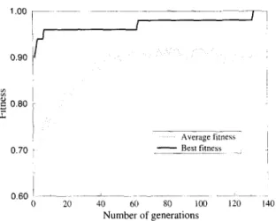
f Average fitness ] Best fitness ] 0 . 6 0 . . . . ~ . . . 0 20 40 60 80 100 120 140 Number of generations

Fig. 1. Best and average fitness values through generations in the stationary inventory.

sions are made by a manager; hereafter we will call the manager the decision maker. The decision maker has the full authority to develop procurement and inventory stocking policies for the items held in the Department. The inventory consists of 145 stationary items.

The decision maker classified the items according to four criteria, as follows:

CI: Annual dollar usage.

C2: Number of requests for the item in a year. C3: Lead time.

Ca: Replacability (0: replaceable, 1: sometimes replaceable; 2: cannot be replaced).

We first asked the decision maker to name ten items from each of the three classes. In order to minimize subjectivity, we also requested the decision maker to make his selection from the characteristic and distin- guishing items. This set of 30 items formed our training set for the GA. The genetic algorithm was run on a population of 100 chromosomes, with Pc = 0.7 and Pm= 0.001. Our genetic algorithm converged on the

training set in the 132nd generation after 9285 function evaluations. During this process GAMIC has performed 4580 crossover operations and 75 mutations. The best and average fitness values in each generation are shown in Fig. 1. The weights learned by GAMIC are as follows: Wl = 0.268, w2 = 0.359, w3 = 0.034,

Table 1

Comparison of classifications made by the GAMIC and AHP with respect to decision maker, on the stationary inventory. Entry in the i-th row and j-th column represents the number of classifications made by decision maker as class i and by the corresponding algorithm as class j

Decision GAMIC AHP

maker A B C A B C

A 26 23 3 0 12 8 6

B 27 1 21 5 11 12 4

C 92 0 1 91 6 9 77

Total 145 24 25 96 29 29 87

w4 = 0.339 and the cut-off points are XAB = 0.347,

XBC = 0.228.

We classified the remaining 115 items using the weights and cut-off values learned by the GA. The decision maker also was asked to classify these test items. The decision maker's classification did not agree with GAMIC on 10 items. The results of the classifications by GAMIC versus the decision maker are given in Table 1.

In order to compare with the AHP technique, the decision maker was asked to pairwise compare the four criteria. In the third attempt the decision maker was able to obtain a consistent matrix. The weights obtained by the AHP technique are as follows: wl = 0.558, w2 = 0.233, w3 = 0.156, w4 = 0.052 and the cut-off points are XAB = 0.157, XBC = 0.113. All 145 items were then classified according to the weights learned by the AHP technique. The results of the classifications by AHP versus the decision maker are given in Table 1. The decision maker did not agree with the classification of 44 items. As a result we conclude that the genetic algorithm method proposed here performed much better than the AHP technique in our test set.

5.2. Explosive inventory

This example involves the items held in the site warehouse of a company that undertakes rock exca- vation tasks using explosives [ 10]. The number of criteria used in the classification of the items in that inventory is larger relative to the previous example inventory:

(8)

36 H.A. Guvenir, E. Erel/European Journal of Operational Research 105 (1998) 29-37

C~: Unit price.

C2 : Number of requests for the item in a year. C3 : Lead time.

C4: Scarcity. C5 : Durability. C6 : Substitutability. C7 : Repearability.

C8 : Order size requirement. C9 : Stockability.

Cl0: Commonality.

The criteria C4 through Cl0 take integer values between 0 and 5. The criteria values are assigned to items in such a way that higher values increase the likeli- hood of an item to be placed in class A.

The characteristics of the 115 items held in the inventory vary significantly. For example, a highly ex- pensive explosive with a short shelf-life (low durability), and a particular size nail with high substitutability, stockability, commonality, and durability are in the same inventory.

The decision maker in this example is the manager of the warehouse, who is the sole responsible person in maintaining the inventory.

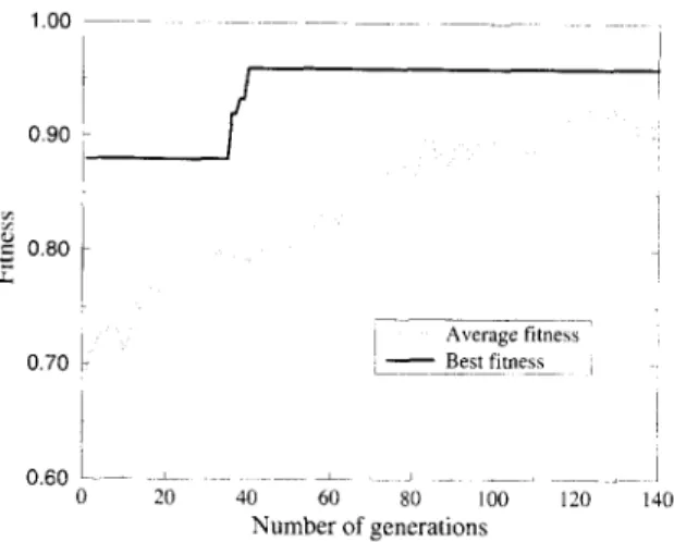
In a similar manner, we first asked the decision maker to name five items from each of the three classes. In order to minimize subjectivity, we also requested the decision maker to make his selection of the above 15 items in such a way that he is absolutely certain about the classes each item belongs to. This set of 15 items formed our training set for the GA. The genetic algorithm was run using the same set of parameters; that is, a population of 100 chromosomes, with Pc = 0.7 and pm = 0.001. Our genetic algorithm converged on the training set in the 340th generation after 24 003 function evaluations. During this process GAMIC has performed 11 888 crossover operations and 427 mutations. The best and average fitness values in each generation are shown in Fig. 2. The weights learned by GAMIC are as follows: Wl = 0.151, w2 = 0.009, w3 = 0.276, w4 = 0.137, w5 = 0.072, w6 = 0.168, w7 = 0.000, w8 = 0.013, w9 = 0.035, wl0 = 0.138 and the cut-off points are XAB = 0.476, XBC = 0.325.

We classified the remaining 100 items using the weights and cut-off values learned by the GA. The decision maker also was asked to classify these test items. The decision maker's classification did not

1.00 . . . .

/

I

0.90 ?

I

;~ 0.80 L~ I

!

! 0.70 0.60 ] Average fitness L Best fitness i I

J

20 40 60 80 100 120 140 Number of generations

Fig. 2. Best and average fitness values through generations in the explosives inventory.

agree with GAMIC on 5 items. The results of the classifications by GAMIC versus the decision maker are given in Table 2.

In order to compare with the AHP technique, the decision maker was asked to pairwise compare the four criteria. In the fourth attempt the decision maker was able to obtain a consistent matrix. The weights obtained by the AHP technique are as follows: Wl = 0.358, w2 = 0.137, w3 = 0.246, w4 = 0.066, w5 = 0.041, W 6 = 0.018, w7 = 0.008, w8 = 0.057, w 9 =

0.043, wl0 = 0.025 and the cut-off points are xnB = 0.33, xBc = 0.15. All 115 items were then classified according to the weights learned by the AHP technique. The results of the classifications by AHP versus the decision maker are given in Table 2. The decision maker did not agree with the classification of 15 items. As a result we conclude that the genetic algorithm method proposed here performed much better than the AHP technique in our test set.

The GAMIC program is coded in the LISP lan- guage. The program took 70 seconds and 151 seconds of CPU time for stationary and explosives inventory examples, respectively, on a SunSparc 20/61 worksta- tion.

(9)

Table 2

Comparison of classifications made by the GAMIC and AHP with respect to decision maker, on the explosives inventory. Entry in the i-th row and j-th column represents the number of classifications made by decision maker as class i and by the corresponding algorithm as class j Decision maker GAMIC AHP A B C A B C A 26 26 0 0 22 4 0 B 24 1 23 0 1 18 5 C 65 0 4 61 0 5 60 Total 115 27 27 61 23 27 65 6. Conclusion

We presented a new approach using genetic algorithms to multi-criteria classification. This approach is based on learning a weight vector of absolute weights of each criteria along with a set of cut-off points. In order to apply a genetic algorithm to the weight learning problem, we proposed a new crossover operator that guarantees the generation of offsprings that are valid representations of weight vectors.

The approach, implemented in a program called GAMIC, is applicable to any multi-criteria classification problem with any number of classes, provided that it is possible to reduce the problem to learning a weight vector along with the cut-off points between classes. We have compared our approach with the classical AHP technique on two sample inventory classification tasks. The classifications made by GAMIC were much closer to the classification made by the decision maker than the one obtained by the AHP technique. We have seen that decision makers are more comfortable in classifying inventory items than com- paring two criteria on a scale of 1 to 9. Therefore, the decision makers' decisions about individual classifications of items are more reliable. The main advantage of the approach employed in GAMIC over the AHP technique is its more reliable input. We believe that the approach presented here is applicable to other classification problems as well.

References

[1] RV. Balakrishnan, V.S. Jacob, Triangulation in Decision Support Systems: algorithms for product design, Decision Support Systems 14 (1995) 313-327.

[2] J.C. Bean, Genetics and random keys for sequencing and optimization, ORSA Journal on Computing 6 (2) (1994)

154-160.

[ 3 ] M.A. Davies, Using the AHP in marketing decision-making, Journal of Marketing Management 10 ( 1 ) - ( 3 ) (1994) 57- 74.

[4] B.E. Flores, D.C. Whybark, Multiple criteria ABC analysis, International Journal of Operations and Production Management 6 (3) (1986) 38-46.

[5] B.E. Flores, D.L. Olson, V.K. Dorai, Management of multicriteria inventory classification, Mathematical and Computer Modeling 16 (12) (1992) 71-82.

[6] D.E. Goldberg, M.R Samtani, Engineering optimization via genetic algorithm, in: Proceedings of the Ninth Conference on Electronic Computation, 1986, 471-482.

[7] D.E. Goldberg, Genetic Algorithms in Search, Optimization and Machine Learning, Addison-Wesley, Reading, MA,

1989.

[8] M. Gulsen, A.E. Smith, D.M. Tare, A genetic algorithm approach to curve fitting, International Journal of Production Research 33 (7) (1995) 1911-1923.

[9] H.A. Guvenir, I. Sirin, A genetic algorithm for classification by feature partitioning, in: S. Forest (Ed.), Proceedings of the Fifth International Conference on Genetic Algorithms, 1993, pp. 543-548.

[ 10] N. Guvenir, Application of AHP to multicriteria inventory classification, M.BA. Thesis, Graduate School of Business Administration, Bilkent University, Ankara, Turkey, 1993. [1 l] J.H. Holland, Adaptation in Natural and Artificial Systems,

MIT Press, Cambridge, MA, 1975.

[12] M.H. Lu, C.N. Madu, C.H. Kuei, Integrating QFD, AHP and benchmarking in strategic marketing, The Journal of Business and Industrial Marketing 9 ( 1 ) (1994) 41-50. [13] T.L. Saaty, The Analytic Hierarchy Process, McGraw-Hill,

New York, 1980.

[14] E.A. Silver, R. Peterson, Decision Systems for Inventory Management and Production Planning, Wiley, New York, 1985.

[15] S. Uckun, S. Bagchi, K. Kawamura, Y. Miyabe, Managing genetic search in job shop scheduling, IEEE Expert, October (1995) 15-24.

[ 16] B. Ulengin, E Ulengin, Forecasting foreign exchange rates: a comparative evaluation of AHR Omega 22 (5) (1994) 505-519.

117] E Zahedi, The analytical hierarchy process - a survey of the method and its applications, Interfaces 16 (4) (1996) 96-108.