OPTIMAL TIMING OF AN ENERGY
SAVING TECHNOLOGY ADOPTION
A Master’s Thesis
by
Mehmet Fatih HARMANKAYA
Department of
Economics
·
Ihsan Do¼
gramac¬Bilkent University
Ankara
OPTIMAL TIMING OF AN ENERGY SAVING TECHNOLOGY
ADOPTION
Graduate School of Economics and Social Sciences
of
·
Ihsan Do¼
gramac¬Bilkent University
by
MEHMET FAT·
IH HARMANKAYA
In Partial Ful…llment of the Requirements For the Degree
of
MASTER OF ARTS
in
THE DEPARTMENT OF ECONOMICS ·IHSAN DO ¼GRAMACI BILKENT UNIVERSITY ANKARA
I certify that I have read this thesis and have found that it is fully adequate, in scope and in quality, as a thesis for the degree of Master of Arts in Economics.
— — — — — — — — — — — — — — — — — — – Assist. Prof. Dr. Hüseyin Ça¼gr¬Sa¼glam Supervisor
I certify that I have read this thesis and have found that it is fully adequate, in scope and in quality, as a thesis for the degree of Master of Arts in Economics.
— — — — — — — — — — — — — — — — — – Assist. Prof. Dr. Tar¬k Kara
Examining Committee Member
I certify that I have read this thesis and have found that it is fully adequate, in scope and in quality, as a thesis for the degree of Master of Arts in Economics.
— — — — — — — — — — — — — — Assoc. Prof. Dr. Levent Akdeniz Examining Committee Member
Approval of the Graduate School of Economics and Social Sciences
— — — — — — — — — Prof. Dr. Erdal Erel Director
ABSTRACT
OPTIMAL TIMING OF AN ENERGY SAVING
TECHNOLOGY ADOPTION
HARMANKAYA, Mehmet Fatih M.A., Department of Economics
Supervisor: Assist. Prof. Dr. Hüseyin Ça¼gr¬Sa¼glam September 2011
In this thesis, we use two stage optimal control techniques to analyze the opti-mal timing of energy saving technology adoptions. We assume that the physical capital goods sector is relatively more energy intensive than consumption goods sector. First, we solve a benchmark problem without exogenously growing en-ergy saving technology frontier. In such a case, the economy sticks either to the initial technology or immediately switches to a new technology, depending on the growth rate advantage compared to the obsolescence and adjustment costs. In the second step, we introduce exogenously growing energy saving technology frontier. The anticipated level of the technology provides incentives to delay the adoption and generates an interior switching time. Finally, we analyze numeri-cally the e¤ects of the speed of adjustment to the new technology, growth rate of technology, subjective time preference and planning horizon on the optimal timing of technology adoption.
Keywords: Optimal Control, Technology Adoption, Energy Saving Technical Progress, Embodiment
ÖZET
ENERJ·
I TASARRUFLU TEKNOLOJ·
I
ADAPTASYONUNUN OPT·
IMAL ZAMANLAMASI
HARMANKAYA, Mehmet Fatih Yüksek Lisans, Ekonomi Bölümü
Tez Yöneticisi: Assist. Prof. Dr. Hüseyin Ça¼gr¬Sa¼glam Eylül 2011
Bu tezde, enerji tasarru‡u teknoloji adaptasyonunun optimal zamanlamas¬n¬analiz etmek için iki a¸samal¬optimal kontrol tekniklerini kullan¬yoruz. Fiziksel sermaye mallar¬sektörünün, tüketim mallar¬sektörüne oranla enerjiye daha fazla ba¼g¬ml¬ oldu¼gunu varsay¬yoruz. Öncelikle, d¬¸ssal geli¸sen enerji tasarru‡u teknoloji içer-meyen temel bir model çözüyoruz. Böyle bir durumda, büyüme oran¬avantaj¬n¬n eskime ve ayarlama maliyetleri kar¸s¬s¬ndaki durumuna ba¼gl¬ olarak ekonominin ba¸slang¬ç seviyesindeki teknolojide kald¬¼g¬n¬ ya da daha yüksek enerji tasarrufu sa¼glayan yeni teknolojiye ba¸slang¬çta geçti¼gini gözlemliyoruz. Ikinci a¸· samada, modele d¬¸ssal geli¸sen enerji tasarru‡u teknoloji ekliyoruz. Böyle bir modelde, öngörülen teknoloji seviyesi, adaptasyonun gecikmesini te¸svik edip bu adaptasy-onunun dahili zamanlarda gerçekle¸smesini sa¼gl¬yor. Son olarak, yeni teknoloji ayarlama h¬z¬n¬n, teknoloji geli¸sme oran¬n¬n, öznel zaman tercihinin ve planlama süresinin teknoloji adaptasyonu optimal zamanlamas¬na etkilerini nümerik olarak inceliyoruz.
Anahtar Kelimeler: Optimal Kontrol, Teknoloji Adaptasyonu, Enerji Tasarru‡u Teknik Geli¸sme, Somutla¸sma
ACKNOWLEDGEMENTS
I would like to express my deepest gratitude to my supervisor, Assist. Prof. Ça¼gr¬ Sa¼glam, who has supported me throughout my thesis with his patience, knowledge and exceptional guidance in all of the stages of my study. I am indebted to him. I would like to thank Assist. Prof. Tar¬k Kara, as one of my thesis examining committee members, who gave his time and provided worthy guidance. I also would like to thank Assoc. Prof. Levent Akdeniz for his interest and helpful suggestions as an examining committee member.
Thanks to TÜB·ITAK and Bilkent University for their …nancial support dur-ing my graduate study.
Special thanks to my graduate friends, for their invaluable smile and close friendship. Not forgetting to my friends, especially Fevzi Y¬lmaz, who have always been there and gave me the moral support during my graduate study. Life would have been too boring without delighted moments spent with them.
I would like to thank my family for being always there with all their love and continuous support, during my graduate study and entire life.
However, while grateful to them, I bear the sole responsibilities for all the mistakes made in the thesis.
TABLE OF CONTENTS
ABSTRACT . . . iii
ÖZET . . . iv
ACKNOWLEDGMENTS . . . v
TABLE OF CONTENTS . . . vi
LIST OF TABLES . . . vii
CHAPTER 1: INTRODUCTION . . . .1
CHAPTER 2: THE BENCHMARK MODEL . . . 6
2.1 The Model . . . 6
2.2 Two Stage Control Approach . . . 9
2.2.1 The Second Stage Problem . . . 9
2.2.2 The First Stage Problem . . . 11
2.2.3 Value of the Optimal t1 . . . 12
2.3 In…nite Horizon Case. . . .14
CHAPTER 3: AN EXOGENOUSLY GROWING ENERGY SAV-ING TECHNOLOGY FRONTIER . . . .16
CHAPTER 4: NUMERICAL ANALYSIS . . . 20
CHAPTER 5: CONCLUSION . . . 25
LIST OF TABLES
1. Values of the benchmark parametrization . . . .20
2. The E¤ect of changes in the technological growth parameter . . . .21
3. The E¤ect of changes in the energy price . . . .22
4. The E¤ect of changes in the adjustment parameter . . . .22
5. The E¤ect of changes in the subjective time preference . . . .23
6. The E¤ect of changes in the planning horizon . . . .23 7. The E¤ect of changes in the share of energy in capital good production . .24
CHAPTER 1
INTRODUCTION
Adoption of cleaner technologies has become one of the most important topics in environment and growth …elds. This stems from the fact that due to scarcity and the pollutant property of energy resources, consumers may shift their demands to goods that are produced with less energy resources and …rms can switch technologies which are using resources more e¢ ciently.
The adoption of cleaner technologies establishes the connection between tech-nology switching and the environmental protection. Cunha-e-sa and Reis (2007) study the optimal timing of adopting a cleaner technology and its e¤ects on the growth rate of the economy in the context of an AK endogenous growth model. They introduce environmental quality to their utility function which increases the utility of the consumption. Boucekkine, Krawczyk and Vallee (2010) study the trade o¤ between economic and environmental bene…ts where the agent can switch to a cleaner technology that is economically ine¢ cient. They introduce pollution to the utility which negatively e¤ects the total welfare. Di¤erently, this thesis examines energy saving technology adoption which is not previously considered and includes the adoption of a new technology in capital goods sector which uses energy more e¢ ciently.
However, technology adoptions are costly due to the e¢ ciency losses and asso-ciated costs of new technologies. Parente (1994) claims that, technology adoptions induce e¢ ciency losses in human and physical capital. There exists a slow learning process in which the economy is unable to produce at its best level. Moreover, when
the economy switches to a new technology, the adoption costs occur via di¤erent mechanisms. Such costs associated with technology adoption are called learning, obsolescence and adjustment costs in the literature. When these are considered to-gether with learning and other costs of new technologies, the following question may emerge: Is it optimal to switch to the new technology or continue with the older one? While trying to answer this question from an economic perspective, the timing of this adoption is also taken into consideration.
The optimal timing of technology adoptions depends on the growth advantages, the speed of learning and the obsolescence costs (see Boucekkine, Saglam and Vallee (2004)). Real income, human capital, the trade between countries and the type of government are among the other determinants of technology adoption according to Comin and Hobjin (2003) which includes their empirical analysis on cross-country technology adoption in the time period from 1788 to 2001. We investigate the e¤ects of some of these determinants on the optimal switching time.
Boucekkine, Saglam and Vallee (2004) studies various adoption problems in the optimal growth framework. They study the optimal timing of switching to new tech-nologies with and without learning behavior. Two stage optimal control techniques are used to determine the switching time. When learning behavior does not exist, the solution will be immediate or never adoption. However, when it is introduced, the economy will switch immediately or choose the delay option. Saglam (2010) also studies the optimal pattern of technology adoption with multiple switches instead of a single switch. They introduce technology-speci…c adjustment cost on the de-preciation parameter to explain the loss of expertise caused by newer technologies. We simply consider the adjustment cost of the new technology similar to Saglam (2010).
The usage of energy resources have been extensively analyzed in the optimal growth literature. Most of these analyses are based on the assumption that phys-ical capital and consumption good use the same technology in production. This assumption implies that the energy intensities of these goods are same. However,
as Perez-Barahona (2007) states, physical capital accumulation usually involves the transformation of raw materials into iron, steel and non-ferrous metals. Transport and storage of goods are also included in physical capital whereas consumption good sector is more related to food, clothes and construction. Azamahoau et al. (2006) shows that energy intensities of physical capital goods are much more higher than consumption goods. They …nd that the ratio between energy consumption and the value added is 0.809 for iron and steel, 0.85 for storage and transport whereas 0.134 in food and tobacco, 0.082 in textile production. Perez-Barahona (2007) uses a type of setting where physical capital accumulation is more energy intensive than con-sumption good. They consider a general equilibrium model consisting of …nal good, physical capital and resource extraction sectors. Within these sectors, they study the implications of assuming di¤erent technologies for physical capital accumulation and consumption.
In this thesis, we use a simple optimal growth model to solve the technology adoption problems in continuous time. Technological progress is assumed to be embodied in capital good production, speci…cally in energy usage. In addition to switching to the new technology, our problem involves obsolescence costs and learn-ing costs integrated in depreciation term. The economy starts with a given initial technological menu and level of embodied technical change in energy saving tech-nology. New technological menu is also available starting from the beginning of the planning horizon. The agent may switch to the new technology or continue to use the current one at any instant of the time. However, new technology is costly as more embodiment in capital sector, speci…cally in energy sector, implies a decrease in the relative price of capital. This decrease induces a rise in the level of resources used in investment which drops the consumption level. The welfare cost of this drop is referred to obsolescence costs as stated in Saglam (2010). In addition to these ob-solescence costs, switching to the new technology induces accelerated erosion e¤ect on physical capital which can be considered as the learning cost of new technology. The loss of expertise after switching is expressed by using associating accelerated
depreciation to the new technology. We want to examine under which conditions and when, the economy would switch to a more e¢ cient energy saving technical progress knowing the obsolescence and learning costs of the switching.
We consider a simple AK type production function in consumption good and Cobb-Douglas type function in capital good sector. Due to AK production function, long term growth is no longer exogenous. Boucekkine et al. (2004) assume that in the new technology case, disembodied technological progress is lower in order to represent the loss of expertise after switching. Di¤erently, we introduce costs of the new technology in the depreciation parameter. In our benchmark model, we assume that the higher level of embodied technical progress is available with a higher depreciation rate because of learning costs. In the extended model, we assume that there exists an anticipated technology adoption and time-varying embodied energy saving technological progress.
In the capital good sector, we consider a capital accumulation rule similar to Perez-Barrahona (2007) which implies that energy intensity of capital good is higher than consumption good. In contrast with Perez-Barrahona (2007), we do not in-clude the extraction sector of energy resource. Instead, energy is assumed to be purchased directly with a given cost function in order to simplify the model. We are able to derive the paths followed by the decision variables analytically which allows us to use two-stage optimal control techniques proposed by Tomiyama and Rossana (1989). By using this approach, we can generate three possible decisions related to optimal timing: immediate adoption, technological sclerosis, i.e., sticking to the initial technology through the planning horizon implying corner solutions and delayed adoption as an interior solution.
The organization of the paper is as follows. In Chapter 2, the benchmark model will be introduced and solved by using two-stage optimal control technique for both …nite and in…nite horizon. The procedure of the two-stage approach and how it works will also be presented. In Chapter 3, we will extend our model by allowing the energy saving technology frontier level to increase throughout the time. We apply
same procedure as benchmark case in order to reach optimal timing of adoption. However, as in many optimal timing problems, we are unable to reach open form analytic solutions. Thus, in Chapter 4, numerical analysis and comparative statics for the parameters of the will take place. Finally, Chapter 5 concludes the paper.
CHAPTER 2
THE BENCHMARK MODEL
2.1
The Model
In this section, we consider an economy inhabited by a representative agent who deals with the problem of technology adoption which tries to maximize the following inter-temporal utility function:
T
Z
0
u(C(t))e tdt
where C is the aggregate consumption and u(:) is assumed to be increasing and concave. We do not analyze any labor dynamics throughout the paper, so population is assumed to be normalized to one and there is no population growth. Time horizon is taken as …nite1 in order to illustrate the sensitivity of optimal adoption timing to
the optimization horizon and denotes the subjective time preference.
For the consumption good sector, we use AK technology which uses physical capital as only input.
Y (t) = A(t)K(t) (1)
where A denotes marginal productivity of capital and K denotes physical capital used to produce consumption good. The …nal good is either consumed or invested
in physical capital or used for purchasing energy, which is used in production of capital good, satisfying the budget constraint:
Y (t) = C(t) + I(t) + f (R(t)) (2)
where I and R denotes investment and energy usage respectively and f is a convex cost function of energy.
Energy saving technological progress is special for our model. Increasing the e¢ ciency of energy usage is the fundamental aim of the problem. By improving energy e¢ ciency, same level of capital good can be produced by low level of energy. The energy intensity of physical capital is higher with respect to the consumption good. To imply this intensity, we assume that physical capital accumulation is a function of energy and investment.2 Energy is purchased directly with a given cost
function. The technology for physical capital uses Cobb-Douglas function with the following accumulation rule:
:
K(t) = (q(t)R(t)) I(t)1 (t)K(t)
Here, q(t) denotes the energy saving technological progress, which is assumed to be constant for this section, (t) denotes the depreciation function and K(0) = K0 > 0
is taken as given. Accordingly, we assume that the energy and the investment are substitutes in physical capital production. Energy is purchased at a price of p relative to the consumption good to be used in capital good production.
There are two technological menus for the economy. The economy starts with ( 1; q1) and another option ( 2; q2) is available starting from t = 0 where q2 > q1
and 2 > 1. The economy can switch to a new technological regime with a more
e¢ cient energy usage in capital production at any instant of time. In contrast to increase in A the rise in q will only a¤ect the capital goods. This rise will decrease the relative price of physical capital which induces a drop in consumption which
is referred as obsolescence cost. Moreover, switching to a more e¢ cient energy saving technology incurs a loss in expertise expressed as an increased depreciation. Switching to a new technology induces accelerated erosion in physical capital and a slow adjustment process for reaching the best productivity level of the technology. Due to this erosion e¤ect the depreciation function after switching is composed of two parts including the technology speci…c adjustment cost of the adoption. The second part is eroded with the speed of as time passes. Put di¤erently, can be expressed as the speed of learning the usage of the new technology. More precisely, we have:
2(t) = + e (t t1) 8t 2 [t1; T ] (3)
where and are positive parameters and adjustment costs are eliminated with a speed measured by the parameter, :
Now, assume that the economy switches to a new technology regime at a date t1. The state equation of capital di¤ers after and before t1 due to the technological
menu change. Before the adoption, i.e., 0 t < t1; the evolution of physical capital
can be written as:
:
K(t) = (q1R(t)) I(t)1 1(t)K(t) (4)
After the adoption, i.e., t1 t < T;the evolution of capital is: :
K(t) = (q2R(t)) I(t)1 2(t)K(t) (5)
where 1(t) = and 2(t) is given as in equation (3). Note that, there is a trade
o¤ between two consecutive regimes. The productivity parameter of energy, q is higher in new technology regime, however, as the depreciation rate increases in the switching time, the capital accumulation is negatively e¤ected. To solve the problem, we can move to the two stage optimal control approach.
2.2 Two Stage Optimal Control Approach
Our optimal control problem can be written as
max R;C;t1 T Z 0 u(C(t))e tdt
subject to the constraints (1); (2); (4) and (5) and given K0 > 0. Due to its dynamic
structure, the problem can be rewritten as:
U (C; t1) = t1 Z 0 u(C(t))e tdt + T Z t1 u(C(t))e tdt
Here, t1 2 [0; T ] denotes the optimal switching time to new technologic regime.
Since, two stage optimal control technique is well suited to our problem, we use this approach to …nd the value of the optimal t1. This approach needs to divide the
problem into two stages and operates in the following way:
2.2.1 The Second Stage Problem
We …rst assume that switching realizes at t1 and the initial capital stock at t1 is
given, namely K(t1) = K1. For this stage we use logarithmic utility function and
try to maximize: U2(K1; t1) = T Z t1 ln(C(t))e tdt
subject to the state equation (5) and free K(T ). In order to simplify the model we take linear cost function for energy. The corresponding Hamiltonian can be de…ned as:
To simplify notation, we will not use time index after this point unless it is necessary. First order conditions can be written as:
HC2 = e t C 2[(1 )(q2R) (AK C pR) ] = 0; HR2 = 2[ q2(q2R) 1(AK C pR)1 p(1 )(q2R) (AK C pR) ] = 0; HK2 = 2 (1 )A(q2R) (AK C pR) 2 = 2 where H2
C, HR2 and HK2 are the …rst order conditions with respect to consumption,
energy and capital respectively and K1 is given. By using …rst order condition for
energy usage we reach:
R(t) =
pAK(t) C(t)
for every t 2 [t1; T ]. Replacing this value on the …rst order condition for consumption
we get the value of co-state variable as:
2(t) = e t C(t)(1 ) 1( p q2 )
Using this equation with the …rst order condition for physical capital, we have:
C(t) C(t) = A (1 ) 1( p q2) 2
From this equation we reach the paths followed by consumption, capital and co-state variable.
C(t) = a1e
At(1 )1 ( p q2 ) +
e (t+t1) t( + )
K(t) = 1e A(t1 t( 1+ ))(1 ) q2p +( 1+e( t+t1) ) t1 t( + ) (1 ) p q2 [a1e At1(1 ) q2p + et et1 ( 1 + ) +et +t1 A(1 ) p q2 + + K 1(1 ) p q2 ]; 2(t) = e At1(1 )1 (q2p ) +t e( t+t1) (1 ) 1(qp 2 ) a1 :
By using the limit condition for the economy, lim
t!T 2(t)K(t) = 0, we can reach
the value of a1 as:
a1 =
e +T +t1 A(1 )1 (q2p ) + +
K1(1 ) qp
2
eT et1 :
By incorporating these values into the integration, we get the value for the optimal welfare in the second stage as U2(K1; t1) which is twice di¤erentiable both
with respect to K1 and t1.
2.2.2 The First Stage Problem
After solving the second stage problem, we now turn to the original problem and rewrite it as: max C;R;t1 U (C; t1) = t1 Z 0 u(C(t))e tdt + U2(K1; t1)
subject to the constraint (4) with given K0and free K1values. To solve this problem,
by using Pontryagin maximum principle and taking K1 and t1 as …xed, we can write
corresponding Hamiltonian as:
and get the paths for consumption, capital and co-state variables as follows:
C(t) = a0e
At(1 )1 ( p
q1 ) t( + )
where a0 is the constant of integration which is unknown.
K(t) = 1e t A(1 ) 1 p q1 (1 ) p q1 a0 et 1 ( 1 + ) + et K0(1 ) p q1 ; 1(t) = et1 (1 )1 (q1p ) + (1 ) 1(qp 1 ) a0 :
By using the continuity condition 2(t1) = 1(t1)for co-state variable at t1 we …nd
a0 as: a0 = eT +t1 A(1 )1 (q1p ) + + K1(1 ) 1+ qp 1 eT et1 :
and by using the continuity condition for capital stock we solve for K1:
K1 = e t1( + ) et1 A(1 ) 1 ( p q1 ) + + eAt1(1 ) 1 ( p q1 ) +T K0 eT 1 :
2.2.3 Value of the Optimal t1
Since t1 exists in the one of the state equation, namely in equation (5), we need to
satisfy the following equations in order to have the interior solution:
@U2(K1; t1) @t1 = H1(K1; t1) + t1 Z 0 @H1 @t1 dt
H2(K1; t1) H1(K1; t1) = t1 Z 0 @H1 @t1 dt + T Z t1 @H2 @t1 dt (6)
In this case, the su¢ cient condition for maximum can be written as:
@H2(K1; t1) @t1 @H1(K1; t1) @t1 < @ @t1 2 4 t1 Z 0 @H1 @t1 dt + T Z t1 @H2 @t1 dt 3 5
Corner solutions may also arise in this situation: (i)Immediate switching: t1 = 0 if
H1(K1; t1) H2(K1; t1) t1 Z 0 @H1 @t1 dt + T Z t1 @H2 @t1 dt when t1 = 0 (7) (ii) Technological sclerosis: The economy will never switch to new technology on [0; T ] if H1(K1; t1) H2(K1; t1) t1 Z 0 @H1 @t1 dt + T Z t1 @H2 @t1 dt when t1 = T (8)
Using the …rst and the second stage problems together, we characterize the con-sumption, capital, energy and co-state variables paths for given K0 and t1. Finally,
in order to determine optimal t1, we use the equation (6) and get the equation that
optimal t1 should satisfy. However, for this case we have no interior solution for t1
such that it belongs to the interval (0; T ). As stated above, corner solutions which are immediate switching or technological sclerosis may arise in this case. If the ex-pression (7) holds at t1 = 0, then the economy will switch immediately to the new
technology. Otherwise, the expression (8) holds at t1 = T, the technology will never
switch to the newer one, i.e. technological sclerosis occurs.
Note that, there is no incentive to switch to the new technological regime in the time interval (0; T ). If the associated costs are to be eliminated su¢ ciently to in-crease the total welfare during the planning horizon, the option of delaying adoption cannot be optimal. In this case, the economy switches to the new technology
imme-diately. Otherwise, if the costs cannot be eliminated su¢ ciently and total welfare is less than no switching case, the economy will never switch to new technology. In this type of model, there is no delaying option of new regime, i.e., delaying adoption will have no bene…t.
The increase in the rate of the energy saving technological progress is associated with an increase in the depreciation rate of the physical capital, which is decreasing with the time up to the initial level. The change in this rate is combined with the costs induced by the loss in expertise, namely learning and obsolescence costs. If the economy switches to new regime and resulting improvement in e¢ ciency is enough to compensate the loss in expertise, the economy will face a higher growth rate and will not delay the adoption.
2.3
The In…nite Horizon Case
In this section, we study the in…nite horizon extension of our benchmark model, i.e., T = 1. For this case, we follow the same steps as in the solution of the benchmark model. The optimization horizon enters to the model in the second stage optimization, so-called new technology problem. Now the limit conditions are replaced by the transversality conditions as when T goes to in…nity:
lim
t!1 2(t)K (t) = 0
As one can easily check this is the unique departure from the benchmark …nite horizon model. In the new technology problem, on [t1;1), paths for consumption,
capital and co-state variable remains same as in …nite case except for the coe¢ cient a1. In this case, a1 can be written as:
a1 = e +t1 A(1 )1 (q2p ) + + K1(1 ) 1 p q2 :
In the old technology problem, the situation is similar to the new technology problem. On [0; t1); paths for consumption, capital and co-state variable remains
same as in …nite case except for the coe¢ cient a0. By using continuity of co-state
variable at t1, we get a0 as:
a0 = e t1 A(1 )1 (q1p ) + + K1(1 ) 1 p q1 :
Also, using the continuity for the physical capital leads
K1 = e
At1(1 )1 (q1p ) + t1( + )
K0:
Now, following the same steps as in the …nite case and by using equation (6) for our problem, we reach the equation that t1 should satisfy. For this case, we have no
interior solution for t1 such that it belongs to the interval (0; 1). Corner solutions
which are immediate switching or technological sclerosis also arise in this case. If the expression (7) holds at t1 = 0, then the economy will switch immediately to the
new technology. Otherwise, the expression (8) holds at t1 =1, the technology will
never switch to the newer one, i.e., the technological sclerosis occurs. Similar to the previous case, there is no incentive to delay the adoption of the new technology.
In this case, we consider the energy saving technology to jump the given constant level. As a result, we …nd that there is no interior switching option for this setup of the model. Accordingly, we introduce exogenously growing energy saving technology in the next section which guarantees interior solution for optimal timing.
CHAPTER 3
EXOGENOUSLY GROWING ENERGY
SAVING TECHNOLOGY FRONTIER
In the benchmark model, we assumed that the technology is constant at switching time. However, the energy speci…c technology level is continually increasing along with time. This situation leads the representative agent to wait for a jump to a higher level of technology by delaying the adoption. In our model, the agent knows the growth in the technology will continue till the end of the planning horizon and make decisions accordingly. At t = 0, the level of the energy saving technological progress is anticipated at any instant of the optimization period.
We consider a linearly increasing technology with a speed of . The available level of energy saving technology at time t is given by q(t) = 1+ t.3 At any t1, the economy may switch to a more e¢ cient energy using technology e¤ecting
the e¢ ciency of capital goods sector positively, where the adopted energy saving technology level will be q(t1) = 1+ t1. As explained in the benchmark model,
this rise in q will only a¤ect the capital goods, in contrast to an increase in A. The rise will induce a drop in consumption which is referred as obsolescence cost. Moreover, switching to a more e¢ cient energy saving technology incurs a loss in expertise which can be expressed as an accelerated depreciation. As a result, the
3See Dogan, Le Van and Saglam (2011). Moreover, exponentially growing technology case,
accumulation rule for the stock of capital for the second stage is:
:
K(t) = [(1 + t1)R(t)] I(t)1 2(t)K(t)
All other assumptions, equations and the parameters remain as in the benchmark model. We will follow exactly the same steps as in the benchmark model. As de…ned in the two stage optimal control approach, we start by de…ning corresponding Hamiltonian for the second stage as:
H2 = e tln(C(t))+ 2(t)[((1+ t1)(R(t)) (A(t)K(t) C(t) pR(t))1 2(t)K(t)]
After writing the …rst order conditions and making necessary calculations in-cluding algebraic operations similar to the benchmark case, we get the paths for consumption, capital and costate variable for second stage are as follows:
C(t) = a1e At(1 )1 ( p +t1 ) + e (t t1) t( + ); K(t) = 1e A(t1 t( 1+ ))(1 ) +t1p +( 1+e( t+t1) ) t1 t( + ) (1 ) p + t1 [a1e At1(1 ) +t1p + et et1 ( 1 + ) +et +t1 A(1 ) p +t1 + + K 1(1 ) p + t1 ]; 2(t) = e At1(1 )1 ( +t1p ) +t e( t+t1) (1 ) 1( +tp 1 ) a1
By using the limit condition for the economy, lim
t!T 2(t)K(t) = 0, we can reach
a1 =
e +T +t1 A(1 )1 ( +t1p ) + +
K1(1 ) 1+ +tp1
eT et1
Again solving the …rst stage problem similar to the benchmark case by taking q(0) = 1and t1 and K1 …xed, we solve the …rst stage problem by using Pontryagin
maximum principle and write the …rst order conditions. By using these conditions we get the results for the …rst stage:
C(t) = a0eAt(1 ) 1 (p) t( + ) K(t) = 1e t A(1 ) 1 (p ) (1 ) p h a0 et 1 ( 1 + ) + et K0(1 ) p i 1(t) = et1((1 )1 (p) + ) (1 ) 1(p) a0
After making heavy algebraic calculations, we will solve for optimal t1 by means
of the continuity and the optimality conditions. The continuity condition states that the co-state variable for …rst stage and second stage at the adoption time will yield the same value, i.e. 1 j
t=t1
(t) = 2 j t=t1
(t). By using this continuity condition, one can …nd a0 as:
a0 =
eT +t1( A(1 )1 (p) + + )K
1(1 ) 1+ p
eT et1
K1 =
e t1( + ) et1(A(1 )1 (p) + ) + eAt1(1 )1 (p) +T K
0
eT 1
Now we can …nd the optimal value of t1. To achieve this, we need to apply
the optimality condition stated by Tomiyama and Rossana (1989) since our state equation is dependent to t1. Solving this for our problem leads optimal value of t1
should satisfy following equation:
e t1 (ln [(t 1 ) ] + 1 ( + )e T ( + )( et1( + ) + eT +t1 ( + ) + eT ( + )( ( + ))) 1 (1 + t1 ) 2 e T ( +2 )(1 ) AeT ( + )( 1 + ) ( p ( + t1 ) (eT ( + + t1 ) et1 ( + + (t1 T + t1 ) ))) + p (1 + t1 )(eT et1 ) )) = 0
Since this equation cannot be solved analytically for t1, thus we make numerical
CHAPTER 4
NUMERICAL ANALYSIS
In this section, we perform the numerical analysis and comparative statics. We analyze how the trade o¤ between technical progress and adjustment costs, i.e., how the optimal value of t1, responds to an exogenous changes of the parameters of the
model. For the benchmark parametrization, we start by taking parameters as given in Saglam (2010). We take = 0:1when there is no adjustment in the depreciation. This value is consistent with the literature as Nadiri and Prucha (1996) estimates this rate between 0.059 and 0.12. Moreover, relative price of the energy is taken as p = 1:5 to make the comparative analysis. We should also take the parameter carefully in order not to make depreciation rate exceed the necessary level for interior switching or not to block the accumulation of capital.
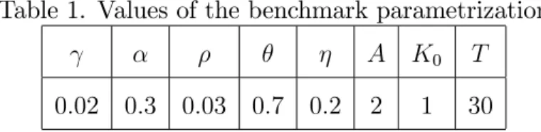
As underlined earlier sections, productivity may not be high at the early stages of the implementation of the new technology. There are many studies examining this ine¢ ciency such as Bahk and Gort (1993). They use panel data from 15 di¤erent industries and estimate that adjustment to new technology is realized within 6 years. Consistent with these learning-by-doing models, we assume that adjustment cost is eliminated with a speed of = 0:7. The other parameters are taken as in Table 1.
Table 1. Values of the benchmark parametrization
A K0 T
0:02 0:3 0:03 0:7 0:2 2 1 30
While …nding optimal technology adoption timing, it should be examined that this value maximizes the total welfare. For this reason we calculate the total welfare
as a function of t1 by taking the given parameters. Our results show that the
value that we …nd is optimal and maximizes the total welfare. When we take the parameters above, we …nd optimal t1 as 11:35 with a total welfare of 167:61 which
is its maximum value and the point where the second derivative is negative.
After …nding the optimal value of t1 and calculating optimal welfare we want to
see the e¤ects of the changes in the parameters. In table 2, the e¤ect of changes in the technological growth parameter, ; in table 3, the e¤ect of changes in price of the energy, p; in table 4, the e¤ect of changes in adjustment parameter, ; in table 5, the e¤ect of changes in the time preference parameter, ; in table 6, the e¤ect of changes in planning horizon, T ; in table 7, the e¤ect of changes in the Cobb-Douglas parameter for energy usage, are presented.
As expected, the increase in the growth rate of energy saving technical progress accelerates the adoption of the new technology. The associated increase in the growth rate advantage reduces the time required for the growth rate advantage to dominate the costs of obsolescence and accelerated depreciation. With the higher values of , instead of waiting switching, one may switch to new technology regime before and the total welfare increases with the increase in .
Table 2. The e¤ect of changes in the technological growth parameter t1 total welf are
0:01 15:23 165:55 0:02 11:35 167:61 0:03 10:27 169:76 0:04 9:71 171:86 0:05 9:35 173:89
The rise in the relative price of energy leads the decrease in the usage of energy in capital good production. In this case, delaying adoption of the new technology will increase the growth rate advantage of the adoption. Thus, when we increase the linear price of the energy, optimal value of t1increases, however when it is compared
to , it has less e¤ect on the optimal timing. Moreover, as one can easily predict, total welfare is decreasing with the increase in price.
Table 3. The e¤ect of changes in the energy price p t1 total welf are
1 11:01 197:32
1:5 11:35 167:61
2 11:63 148:69
2:5 11:88 135:37
3 12:10 125:12
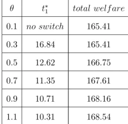
An increase in accelerates the adjustment to the new technology so that increase in will decrease the adoption time. The rise in will eliminate the e¤ect of erosion in capital faster. However, for su¢ ciently small values of , the agent would never switch to new technology and face a technologic sclerosis. Change in does not have signi…cant e¤ects on the total welfare.
Table 4. The e¤ect of changes in the adjustment parameter t1 total welf are
0:1 no switch 165:41 0:3 16:84 165:41 0:5 12:62 166:75 0:7 11:35 167:61 0:9 10:71 168:16 1:1 10:31 168:54
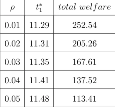
The e¤ect of the time discounting parameter on the pattern of technology adop-tions can be seen in Table 5. It is observed that if the impatience rate is higher, the economy tends to delay the adoption. As increases, the delay in the adoption of the more e¢ cient technology occurs due to the obsolescence costs. With our parameter setting, as increases, the advantage of growth rate of new technology is dominated by the obsolescence costs.
Table 5. The e¤ect of changes in the subjective time preference t1 total welf are
0:01 11:29 252:54 0:02 11:31 205:26 0:03 11:35 167:61 0:04 11:41 137:52 0:05 11:48 113:41
Now, we consider the optimal pattern of technology adoption shifts in response to the changes in the planning horizon. It is clear that longer planning horizons provides an incentive to delay the adoption to have more from the growth rate advantage. As it is proven in Boucekkine et al. (2004), longer planning horizons lead delays in the adoption time of new technology. On the other hand, if the horizon is short enough, the agent would stick to the initial technology and end up with technological sclerosis.
Table 6. The e¤ectof changes in the planning horizon
T t1 total welf are
10 no switch 21:82
30 11:35 167:61
50 15:38 354:16
70 19:13 518:10
1 30:29 891:46
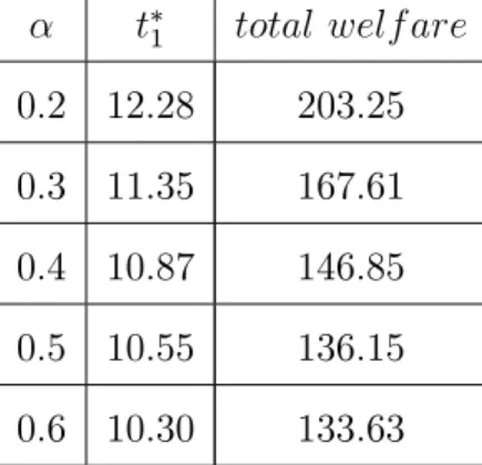
The e¤ect of changes in the share of the energy in capital good production is presented in Table 7. If the share of energy gets higher, optimal adoption time decreases which enables the economy to utilize more from the e¢ cient energy usage.
Table 7. The e¤ect of changes in the share of energy in capital good production t1 total welf are
0:2 12:28 203:25 0:3 11:35 167:61 0:4 10:87 146:85 0:5 10:55 136:15 0:6 10:30 133:63
Finally, the initial level of capital stock, K0 and the level of disembodied
tech-nology, A do not change the optimal adoption timing whereas any increase in initial capital stock level yields a greater level of total welfare certainly. In addition to these comparative statics, we observed that the main factor that a¤ects the adop-tion is the obsolescence cost and adjustment cost due to loss in expertise caused by the embodied technological change. The gain from the rate of this change is associated with a reduction in the price of energy, also in capital, so that more resources are supplied to capital production and consumption level drops. If the adoption is delayed too much, the obsolescence cost gets higher and more drop in consumption is realized. Therefore, it is not optimal to devote more time for waiting later technologies in order to utilize the advantages of newer technology.
CHAPTER 5
CONCLUSION
In this study, we have applied two stage optimal control techniques to solve the optimal adoption problem in a model including energy usage and endogenous de-preciation. We have …rst solved a benchmark model without exogenously growing energy saving technology. To do so, we derived necessary conditions of optimality for two stage optimal control problems in which the switching time appears in the state equation. In this case, delaying the adoption is never optimal. If the growth advantage of the technology adoption is higher than the obsolescence costs and ad-justment costs associated with the depreciation, the economy switches immediately; otherwise, it sticks to the initial technology and technologic sclerosis occurs.
In the second step, we have introduced exogenously growing energy saving tech-nology to the benchmark model. We stated the optimality conditions in this setup and reached the equations that value of the optimal timing should satisfy. Although, we cannot derive the open form analytical optimal adoption timing, we showed nu-merically that interior solution for optimal timing is attained. We also provided numerically the e¤ects of the planning horizon, growth rate of technology, discount-ing parameter, speed of adjustment, share of energy in capital good production and initial level of capital stock on the optimal pattern of the technology adoption. We …nd that increase in speed of adjustment decreases the optimal adoption time. Moreover, any technology growth rate increase also decreases this time. However,
increasing the planning horizon of the model delays the adoption to get more bene…ts from increasing technology frontier.
Further extensions could be considered by applying multi-stage optimal control which allow technology switches. Also, energy sector could be included covering extraction processes and stock levels. Moreover, the damages and the harmful e¤ects of pollutant energy resources could be added to the analysis. Finally, by increasing the number of agents, the interactions among agents could be analyzed..
BIBLIOGRAPHY
Azomahou, T., Boucekkine, R. and Nguyen Van, P. 2006. “Energy Consumption and Vintage Effect: A Sectoral Analysis,” Mimeo.
Boucekkine, R., Saglam, C. and Vallee, T. 2004. “Technology Adoption Under Embodiment: A Two Stage Optimal Control Approach,” Macroeconomic
Dynamics 8: 250-271.
Boucekkine, R., Krawczyk, J. and Vallee, T. 2011. “Environmental Quality Versus Economic Performance: A Dynamic Game Approach,” Optimal Control
Applications and Methods 32: 29-46.
Bahk, B. and Gort, M. 1993. “Decomposing Learning by Doing in New Plants,”
Journal of Political Economy 101: 561-583.
Comin, D. and Hobjin, B. 2004. “Cross Country Technology Adoption: Making the Theories Face the Facts,” Journal of Monetary Economics 51(1): 39-83.
Cunha-e-sa, A.M., Reis, A.B. 2007. “The Optimal Timing of Adoption of a Green Technology,” Environmental and Resource Economics 36: 35-55.
Dogan, E., Le Van, C. and Saglam, C. 2011. “Optimal Timing of a Regime Switching in Optimal Growth Models: A Sobolev Space Approach,” Mathematical Social
Sciences 61(2): 97-103.
Karasahin, R. 2006. “Effects of Endogenous Depreciation on the Optimal Timing of Technology Adoption,” Unpublished Master’s Thesis. Bilkent, Ankara: Bilkent University.
Nadiri, M.I. and Prucha I.R. 1996. “Estimation of the Depreciation Rate of Physical and R&D Capital in the U.S. Total Manufacturing Sector,” Economic Inquiry 34: 43-56.
Parente, S. 1994. “Technology Adoption, Learning by Doing and Economic Growth,”
Journal of Economic Theory 63: 346-369,
Perez-Barahona, A. 2007. “Capital Accumulation and Non-renewable Energy Resources: A Special Function Case,” CORE Discussion Paper, No: 2007-8. Saglam, C. 2010. “Optimal Pattern of Technology Adoptions Under Embodiment: A
Multi-stage Optimal Control Approach,” Optimal Control Applications and
Tomiyama, K. and Rossana, R. 1989. “Two Stage Optimal Control Problems with an Explicit Switch Point Dependence: Optimality Criteria and an Example of Delivery Lags and Investment,” Journal of Economic Dynamics and Control 13: 319-337.