BIT 38:1 (1998), 127-150
A P E N A L T Y C O N T I N U A T I O N M E T H O D F O R T H E
S O L U T I O N OF O V E R D E T E R M I N E D L I N E A R
S Y S T E M S *
MUSTAFA C. P I N A R 1 and SAMIR ELHEDHLI 2
1 Department of Industrial Engineering, Bilkent University Ankara 06533, Turkey. email: mustafap•bilkent.edu.tr
2 Graduate Program in Management, McGiU University Montrdal H3VIG3, Canada. email: elhedhlsOmanagement.mcgill.ca A b s t r a c t .
A new algorithm for the ~oo solution of overdetermined linear systems is given. The algorithm is based on the application of quadratic penalty functions to a primal linear programming formulation of the ~ problem. The minimizers of the quadratic penalty function generate piecewise-linear non-interior paths to the set of goo solutions. It is shown that the entire set of ~ solutions is obtained from the paths for sufficiently small values of a scalar parameter. This leads to a finite penalty/continuation algorithm for ~ problems. The algorithm is implemented and extensively tested using random and function approximation problems. Comparisons with the Barrodale-Phillips simplex based algorithm and the more recent predictor-corrector primal-dual interior point algorithm are given. The results indicate that the new algorithm shows a promising performance on random (non-function approximation) problems.
A M S subject classification: 65K05, 65D10.
Key words: ~o~ optimization, overdetermined linear systems, quadratic penalty func- tions, characterization.
1 I n t r o d u c t i o n .
T h e p u r p o s e of this paper is to give a new finite a l g o r i t h m for the problem
min I l A x - bi]oo-- min m a x l a T x - bil x E R n x E R n i = l . . m
where A E T~ m• is a s s u m e d to have r a n k n with no rows or columns identically zero, a n d b E ~ m . It is well-known [19] t h a t [e~] is equivalent t o the following linear p r o g r a m
min
[LINFLP] s.t.
with the c o r r e s p o n d i n g dual problem
Y A x - y e <_ b A x + y e > b,
128 MUSTAFA C. P I N A R AND SAMIR ELHEDHLI
m a x bT (v -- u)
[LINFLD] s.t. A T ( v -- u ) = 0
eT(u + v) ---- 1
U , V ~ 0
where e is an m-vector with all components unity.
The problem has a wide range of applications, including time series, function approximation and data fitting analysis. As a result, efficient ways to solve it were the subject of many papers (see for example [18]). The first attempts seem to have been made by statisticians as the problem arises frequently in data fitting analysis. More efficient ways, however, were designed when it was realized that the problem is equivalent to a linear program, and, hence it can be solved via any linear programming method. The first numerically stable algorithm for the solution of the ~ problem via the Stiefel exchange method was given by Bar- tels and Golub [1]. Barrodale and Phillips [2] designed a simplex method that exploits the special structure of the coefficient matrix. Alternatively, Bartels, Conn and Charalambous [3] used a direct nondifferentiable descent method. After Karmarkar's outstanding paper which started the area of interior-point methods, Ruzinsky and Olsen [17] used the same ideas to design a polynomial algorithm for the g~ problem. Coleman and Li [6] used a formulation of the ~ problem based upon the null space of A T to propose a globally and quadrati- cally convergent algorithm. Later, subsequent developments in the interior-point area led to the method of Zhang [19], where the predictor-corrector primal-dual interior point approach was adapted to the linear ~oo problems. Zhang's inte- rior point algorithm also possesses local quadratic convergence properties under nondegeneracy assumptions.
The approach of the present paper is based upon recent ideas of Pmar [16] where a quadratic penalty function method was developed to solve a standard dual linear program with only inequality constraints. This was inspired by re- lated work from Madsen and Nielsen [11] and Madsen, Nielsen and Pmar [13] where the gl solution of overdetermined linear systems was studied and later applied to linear programming. However, the ideas of [11, 13] are based on a smoothing approximation of the ~1 function, which is different from the subject of the present paper.
The new method consists of solving a quadratic penalty subproblem for smaller and smaller values of a scalar parameter. In theory, a solution to the original problem could be obtained from a solution to the unconstrained problem when the parameter tends to zero. However, the key to a stable and efficient algorithm is that the parameter tends to zero in a numerically well-defined manner. This is a consequence of the fact that there is a threshold value where optimal solutions to the original problem can be found from the solutions of the penalty problem by solving a linear system. This property is essential both for the efficiency and the numerical stability of the designed algorithm. The algorithm generates a sequence of non-interior iterates that satisfies primal feasibility only upon termination. The purpose of the present paper is to specialize the ideas of [16] to the ~ problem. In particular, we describe the properties of the quadratic penalty function as applied to this problem. Although these results are obtained
A PENALTY METHOD FOR LINEAR MINIMAX PROBLEMS 129
from the analysis of [16], mutatis mutandis, they are reiterated because (1) the ideas of [16] are fairly recent and not well-known, (2) we wish to make the paper self-contained. We redefine the penalty algorithm in the context of the linear too problem and prove its finite convergence. The algorithm is implemented in a software system referred to as LINFSOL, extensively tested, and is compared with the Barrodale-Phillips simplex algorithm and the predictor-corrector interior point algorithm of Zhang.
Our algorithm is not the first penalty function algorithm to be proposed for t ~ problems. Joe and Bartels [9] and Bartels, Conn and Li [4] both used an exact nondifferentiable penalty function approach to solve the problem. Joe and Bartels use the dual formulation of the problem to apply the exact penalty function whereas Bartels, Corm and Li use a primal approach. Our ideas differ from the above in three important aspects:
. We use a differentiable quadratic penalty function which was long forgotten due to potential numerical instabilities. To the contrary, we demonstrate the numerical stability and efficiency of this approach.
2. We utilize a finitely convergent Newton method to solve the penalty sub- problems.
. We exploit the piecewise linear dependence of the minimizers of the penalty function on the penalty parameter to devise a penalty continuation algo- rithm.
The rest of the paper is organized as follows. In Section 2 we will expose the fundamental properties of quadratic penalty functions applied to the too problem. In Section 3 we will present the penalty continuation algorithm based on these properties. Section 4 is devoted to the finite convergence analysis. Finally, in Section 5 we give experimental results.
2 A q u a d r a t i c p e n a l t y f u n c t i o n a p p r o a c h .
Let us consider the following quadratic penalty function
F(x, y,
t) : Sy -{- XrlT(X, y)O1 (x, y)r 1 (x, y) -}- I r T ( x , y)O2(X, y)r2(x,y),
where r l ( x , y ) = A x - y e - b and r2(x,y) = A x + y e - b and 0 1 ( x , y ) and 02(x,y) are m x m diagonal matrices such that 01 = diag(Ol), 02 = diag(02) with 1 i f a T x - - y > b i 91, (x, y) = 0 otherwise, and 1 i f a T x + y < b i 9:,, (x, y) = 0 otherwise.130 MUSTAFA C. PINAR AND SAMIR ELHEDHLI
[LINFCP]
min F ( x , y , t )
x E R n , y E R
for decreasing values of t. It is well-known that the unconstrained minimization
of F(x, y, t) is well defined [5].
For ease of notation let z be the n + 1 vector with zi -- xi ,i = 1 , . . . , n and zn+l -- y, and denote by X the set of optimal vectors z to [LINFLP], and by
Mt the set of minimizers of F ( x , y, t) for a fixed value of t. Let also zt = (xt, Yt) denote a minimizer of F ( x , y, t).
2.1 Properties of F and its minimizers.
In this section, we give a characterization of the set of minimizers of F for fixed t > 0. It is obvious that F(x, y, t) is composed of a finite number of quadratic
functions. In each domain 79 C_ R n+l where 01(x,y),O2(x,y) are constant F
is equal to a specific quadratic function. These domains are separated by the union of hyperplanes
B - - { ( x , y ) e R n + i ; 3 i : a T x - - y - - b i = O V a T x T y - - b i = O } .
So, for a given pair (x, y), the corresponding binary vectors 01 (x, y), 02 (x, y) are found, and F is represented by Qo on the subset,
Co = d { ( ~ , 0 ) ~ Rn+l;01(~,O) = 01 ^ 02(~,0) = 02},
where Q0 is defined as follows:
Qa(Sc, O, t ) = F ( x , y, t) + F T (:~ -- x) + F T (O -- y)
- x)TFxx( - + - y)TF (O - y )
1 ^
- F x , ( O - y ) + - y ) r F , -
with
OF(x, y, t) _ t + e T ( O l q- 02)ey + eT(02 -- O l ) A x + e T ( O l -- O2)b,
Fu - Oy
OF(x, y, t) _ A T ( o 2 _ O1)ey + AT(01 A- 0 2 ) A x - AT(01 d- 02)5,
Fx = Ox
Fxy - 0 2 F ( x ' y ' t ) -= AT(02 -- 01)e,
-- OxOy 0 2 F ( x ' y ' t ) = e T ( 0 2 - - O1)A, Fvx -- OyOx 0 2 F ( x , y , t) _ A T ( o 1 A- Oe)A, F~x - Ox 2 02F(x, y, t) _ eT(O 1 -t- 02)e. Fuu - Oy 2 F.
We refer to the gradient as the (n + 1) vector [F,], and the Hessian as the
[F** F|
A P E N A L T Y M E T H O D F O R L I N E A R M I N I M A X P R O B L E M S 131
be written as j T O A where J - - - [A Ae e] and O = [ol o] We also denote by ' 0 0 2 " Af(P) or No the null space of P . Let b = [~b]. Then the necessary condition for a minimizer zt of F can be written compactly as
(2.1)
-ten+l + ATOD = Pztwhere en+l denotes an n + 1 dimensional vector with a 1 at position n + 1 and
zero elsewhere. In the algorithm of Section 3 we do not form the matrices A, O and P , neither the vector b. These quantities are introduced here to facilitate notation in the analysis.
Now, consider the dual problem to [LINFCP]:
max b T ( v - u) - ~(vTv + u T u )
[PD] s.t. AT(v -- u) = 0
eT(u + V) = 1
U~u ~_O.
As a consequence of strict concavity the above problem has a unique optimal solution and it can be shown that any minimizer (xt, Yt) of F is related to the unique optimal solution (ut, vt) by the identities:
1
(ut)i = - max{0, rli(Xt, Yt) } t
1
(vt )i = - - min{0, r2i(xt, Yt) } t
for i = 1 , . . . , m . This implies the following result.
LEMMA 2.1. 01(xt,Yt) and 02(xt,Yt) are constant for (xt,Yt) E Mr. Fur- thermore aTxt -- Yt -- bi is constant for 01~ = 1 and aTxt + Yt -- bi is constant for 02~ = 1 Vi = 1 , . . . , m .
Following the lemma, the notation 01 (Mr), 02 (Mr) is used instead of 01 (xt, Yt),
02(xt,yt) for (xt,Yt) E Mr. The function F ( x , y , t ) is convex, and hence
the solution set Mt is convex. Now, let Jo = {i101~ = 0 A 02, = 0} and T)o = {z = (x,y) E R'~+llaTx -- y <_ bi A aTx + y > bi A i E Je}. The following
characterization of Mt can be obtained from the previous development.
COROLLARY 2.2. Let zt E Mt and O1 = O l ( M t ) , 0 2 = 0 2 ( M t ) . Then, i t -- (zt +No) n/)o.
Obviously, Mt is a singleton if Af0 consists of the null vector. 2.2 Behavior of the minimizers as a function of t.
The purpose of this section is to show how the solution set Mt of F ( x , y, t)
approximates the solution set X of [LINFLP] as t tends to zero. We begin with a basic lemma. For convenience of notation let Q = OA = O [A A ee]. Clearly,
132 MUSTAFA C. P I N A R A N D S A M I R E L H E D H L I
LEMMA 2.3. Let zt E Mt and 81 = O l ( M t ) , 0 2 ---- 0 2 ( M r ) . Then, the foUowing system is consistent:
(2.2) Pdz = e n + l .
The proof can be obtained by setting the gradient of F at zt equal to zero
and reducing (2.2) into the normal equations corresponding to an overdetermined system.
Let dz be a solution to (2.2). It is straightforward to verify that zt + tdz is
the least squares solution to the overdetermined system of linear equations
(2.3) Qhz = b.
To see this, it suffices to insert Pdz = e , + l in ten+l + P z t = QT~ to get tPdz + P z t = QTy. This implies that QTQ(zt + tdz) = QTy.
LEMMA 2.4. Let zt E Mt and 01 -- 01(Mt),82 = 02(Mr). If the overdeter- mined system (2.3) is consistent then
(2.4) ~Ox(Axt - y t e - b) = - O x ( Adx - dye)
(2.5) 1 0 2 ( A x t + yte - b) = -O2(Adx + dye)
for any solution d~
=(dx, dy) to (2.e).
PROOF. We know that zt + tdz is the least squares solution to the overdeter-
mined system of linear equations Qhz = b. If this system is consistent, zt + tdz
solves Qhz = b. Therefore, we get
0 2 A 02e yt + tduJ b "
O1
0 ]
Premultiplying both sides by 0 02 k = 1, 2, we getand using the fact that 02 = Ok,
02 A 02e Yt + tdu J 02b "
[]
Next, let dz solve (2.2) and assume that 01 (xt + edx, yt + edu) = 01 and 02(xt+edx,yt+edu) = 02, i.e., zt+edz = (xt+edx,yt+edu) E Co for some e > 0.
The linear nature of the problem implies t h a t zt + 6dz = (xt + 6dx, Yt + 6du) E Co
for 0 < 5 < e. Therefore, using the necessary condition for a minimizer of F we get
-ten+l + ATOb = P z t ~ tPdz + P z t = . 4 T O b
A P E N A L T Y METHOD F O R L I N E A R MINIMAX PROBLEMS 133 COROLLARY 2.7.
81
= e l ( M ~ ) , 82 =(2.7)
(2.8) where d~ = drHence, zt + 6dz = (xt + 6dx,yt + 6d u) is a minimizer of F ( x , y , t - 5). Using Corollary 2.2, we have the following result.
LEMMA 2.5. Let zt E Mt and 01 = 01(Mr),02 = 02(Mr). Let dz solve (2.2). I f Ol(xt + edx,yt + ed u) = 01 and 02(xt + edx,yt + edr) = 02 for e > 0 then Ol(xt + 6dz,yt + ~d u) = 01 and 02(xt + 6dx,yt + 6d r) = 02 and
Mr-6 = (zt + 6dz + Ale) f3 De, f o r O < 5 < e .
Although t is a continuous parameter, there is only a finite number of binary vectors 01 and 02. Furthermore, the previous lemma ensures that whenever there exists tt, t2 where 0t (xtl, Ytl ) = 01 (xt2, Yt2) and 02 (xtl, Yn) = 02 (xt2, Yt:) we have 01(xt,Yt) = Ol(Xt,,Ytl) and 02(xt,yt) = Ou(xtl,ytl) for all t e [tl,t2]. As a consequence, 81(Mr) and 02(Mr) are piecewise constant functions of t. Hence, as t tends to 0, 81 and 82 should remain constant in a neighborhood of 0. That is, there exists a positive value of t, say to, such that 81 and 82 remain constant for 0 < t _< to. Therefore we have the following result.
THEOREM 2.6. There exists to > 0 such that 81(Mr) and 82(Mr) are con- stants for 0 < t < to. Furthermore, i] 81(zt +6dz) = 81(Mr) and 82(zt +6dz) = 82(Mr) then
M t - ~ = (zt + ~d~ + Afo) n l)o,
for 0 < 5 < t < to, where dz solves (2.2).
Now, for zt 9 Mt and 81 = ~1(Mt),82 = O2(Mt), let us define
1
(2.6) u t = 01rl(xt,Yt), and v t = - ~ O 2 r 2 ( x t , Y t ) .
Recalling the necessary optimality conditions for a minimizer, we have t - e T O l r l ( x t , Yt) + eTO2r2(xt,Yt) = 0, which implies that eT(ut + vt) = 1, and A T O l r l ( x t , Y t ) + AWO2r2(xt,Yt) = 0 implies that AT(vt - ut) = O. Further- more, (ut,vt) has all components nonnegative. Therefore, (ut,vt) is feasible for [LINFLD]. Now, we give the following important corollary to the previous theorem.
Let 0 < t < to where to is given in Theorem 2.6 and let 82(Mt). Then
Olr1( +td ,y +td ) = 0,
+td ,y +td ) = 0,
is any solution to (2.2). Furthermore,(2.9)
1 O l r l ( x t , y t ) = - O l ( A d x - d r e ),1
(2.10) 702r2(xt,yt)
= -O2(Adx +dre/,
134 M U S T A F A C. P I N A R A N D S A M I R E L H E D H L I
PROOF. Let zt-~ E Mt-~ for 0 < 5 < t. By Theorem 2.6, there exists d~ that solves (2.2) such that z t - ~ = zt + 5dz. Hence, there exists d* that solves (2.2) such that zt + 5d* E M~_~ for all 0 < 5 < t. Now, it is well-known (see e.g., [8]) that lira l r T ( x t , Y t ) O l r l ( x t , Y t ) + ~ r T ( x t , Y t ) O 2 r 2 ( x t , Y t ) = O. t--+o Therefore, we get O l r l ( x t + t d * , y t + t d y ) ---- O, 0 2 r 2 ( x t + td*x,yt + tdu) = O.
Any solution dz of (2.2) can be expressed as dz = dz + r/z where r/z = [~:] E Af(P). However, we have
P~?~ = O ~ Q~?z = O ~ 0 2 A 0 2 e ~y
Inserting this in the above two equations, we get equalities (2.7) and (2.8). Equalities (2.9) and (2.10) follow from Lemma 2.4 since (2.7) and (2.8) imply
that (2.3) is consistent. []
The corollary indicates that the residuals corresponding to the violated in- equalities approach their optimal values in a well-conditioned manner as t de- creases to zero. As we shall see in Section 3, the behaviour of violated residuals is the driving force of the penalty continuation method. Now, we are in a position to give a new characterization of t h e / ~ solutions.
THEOREM 2.8. Let 0 < t ~ to, where to is as given in Theorem 2.6 and let
81 = 81(Mr), 82 = 82(Mr). Let zt E M t and dz solve (2.2).Then
where and X - Mo, Mo = (zt + tdz + Ale) N De, 1 1 u* = ~ 0 1 r l ( x t , y t ) ; v* ---- ---~02r2(xt,Yt) solve [LINFLD].
PROOF. Let z0 E M0. Then there exists a solution ~ to (2.2) such that
zo = z t + t ~ . By Corollary 2.7, we have O l r l ( x o , Y o ) = 0 and 02r2(xo,Yo) = O. Now, using the fact that (u*,v*) is dual feasible (i.e., e T ( u * + v*) = 1 and
A T ( v * -- u*) ---- 0) we get: Y0 = Y0 + 0x0
= yToeT(u* + v*) + x T A T ( v * -- U*)
= ( - - x T A T + e T y T + bT)u * + (XTo A T + e T y T -- bT)v * + bT(v * -- u*)
1 T
= - 7rl (Xo, y o ) O l r l (xt, Yt) - ~r T (Xo, yo)O2r2 (xt, Yt) + bT(v * -- u*)
A P E N A L T Y M E T H O D F O R L I N E A R M I N I M A X P R O B L E M S 135
This shows that Zo and (u*, v*) are optimal in their respective problems. Since this holds for any Zo E Mo, Mo C_ X .
If Mo is a singleton, then the proof is complete. Assume otherwise and let z = (x,y) E X . By feasibility, we have A x - y e < b and A x § > b. Fur- thermore, (x,y) is complementary to (u*,v*) which implies that 0 1 r 1 ( x , y ) = 0 and O2r2(x, y) = 0. This further implies
Ole O2e ] [bb]"
Now, using the above and the necessary condition (2.1) for a minimizer of F (zt minimizes F(x, y, t) ) we have
P ( z - zt)
I
= ten+l - 01e O2e + Ole O2e = ten+l
Thus (z - zt)/t is a solution to (2.2). We have shown that z E zt + tdz + Afo. Now observing that z E Do by virtue of feasibility the proof is completed.
Clearly, X is a singleton if Ale consists of the null vector. 2.3 Extended binary vectors.
In this section, we give some further results that are useful in the design of the algorithm and its finite convergence analysis. We define the following "extended binary vector",
1 i f a T x - - y > b i { 1 i f a T x + y < b i
~1, (x, y) = 0 otherwise and ~2, (x, y) = 0 otherwise.
We also define the "active set" of indices
A(x, y) = {i1 1, (x, y) = 1} u {i1 2, (x, y) = 1}.
Extended binary vectors differ from the binary vectors used thus far only for those points that belong to B. However, this difference leads to an enlargement of the set of violated inequalities, and brings the matrix P closer to having full rank. This enlargement is instrumental in the finiteness proof of the modified Newton used to solve the penalty subproblems. This is discussed in Section 3.1. Now, we analyze the behaviour of the set of extended binary vectors associated with the set of minimizers of F(x, y, t) in the range (0, to] where to is as defined in Theorem 2.6. This is important in establishing the finite termination property of the penalty algorithm defined in Section 3.
Denote by S(Mt) the set of all distinct extended binary pairs of vectors cor- responding to the elements of Mr. In other words, for any (xt,yt) E Mr, (~1 (xt, Yt), ~2(xt, Yt)) e S ( M t ) . We have the following result which is a conse- quence of linearity.
136 MUSTAFA C. PINAR AND SAMIR ELHEDHLI
LEMMA 2.9. If S ( M t l ) = S(Mt2) where 0 < t2 < tl then S ( M t , ) = S(Mt2) = S(Mt) for t2 < t < tx.
Now, as 01(Mr) and 02(Mr) remain constant in (0,to], and the number of
extended binary vectors is finite, the previous lemma ensures that S(Mt) can-
not keep changing infinitely as t approaches 0. Hence, we have the following theorem.
THEOREM 2.10. There exists ~ such that S(Mt) is constant for t E (O,t-)
where 0 < t < to.
For t E (0,t-) let (xt,Yt) E Mt with 01 = ~l(Zt,Yt) and 02 = ~2(:gt,Yt) 9
Consider the system:
(2.11) Pdz = en+l
where
[ AT~}IA + AT~}2A -AT~}ae + AT~}2e ]
P = _eT~}IA + eT~}2A eTOle + eTO2e 9
This is a consistent system of linear equations as shown in Lemma 2.3. By Theo- rem 2.10 there exists (xt,Yt) E Mt such that ~I(Xt,Yt) = ~1 and ~2(Xt,Yt) ---- ~2 for all t E (0,t-). This implies that there exists dz that solves (2.11) such that zt+hdz E Mr-6 for all 5 E [0,t). Now, as t approaches 0, it is well-known (e.g., [8]) that both O l r l ( x t , Yt) and O2r2(xt, Yt) tend to zero. Therefore, we have
O l r l (Xt "1- tdx, Yt + tdu) = O, 0 2 r 2 ( x t + tdx,yt + td~) = O.
By continuity of rl and r2, we have that rli(Xt + tdx,yt + tdy) < 0 for all indices i such that /~1i = 0 and r2i(xt + tdx,yt + td~) > 0 for all indices i such that 02i = 0. This implies that (xt + tdx,yt + tdv) is a feasible point for [LINFLP]. Let u* = l O l r l ( x t , y t ) and v* = - ~ O z r 2 ( x t , y t ) . Since (u*,v*)
is a feasible solution of [LINFLD] and (xt + tdx,yt + tdu) is complementary
to (u*,v*) and is feasible in [LINFLP], it follows that (xt + tdx,yt + td~) and (u*, v*) solve [LINFLP] and [LINFLD], respectively. Clearly, if the solution to (2.11) is unique, d~ = (d~,d;) say, then (xt + td*x,yt + td;) solves [LINFLP]. Since dz can be replaced by dz + 7lz = (d, + ox,d~ + rl~,) where r/z E A/'(P), it follows that
O l r l ( x t -t- tdx,yt + td~) = O,
~}2r2(xt + tdx,yt + td~) = 0
for any solution dz of (2.11). Thus we have the following theorem.
THEOREM 2.11. Let t E (O,t-) and (xt,Yt) E Mt with /~1 = ~l(Mt) and
~2 = 02(Mr). Also, let u* = ~ O l r l ( X t , Y t ) 1 - and V* = - 1 0 2 r 2 ( x t , Y t ) . Then,
(2.12) Olrl(xt + tdx,yt + td~) = O,
(2.13) ~)2rz(xt + td~,yt + td~) : 0
for any solution dz = (dx,d~,) to (2.2). Furthermore, if dz is unique or rl(xt + tdx,yt + tdy) < 0 and r2(xt + tdx,yt + tdu) >_ 0 then (xt + tdx,yt + td~) solves [LINFLP].
A P E N A L T Y M E T H O D F O R L I N E A R M I N I M A X P R O B L E M S 137
3 The penalty algorithm.
Based on the analysis given in the previous sections, a penalty algorithm for ~or problems is designed. The algorithmic ideas are mainly motivated by the results of Theorem 2.11 and Lemma 2.5. For t sufficiently small (t E ( 0 , t ) ) , the point
zt + tdz and the dual pair (u*,v*) as defined in Theorem 2.11 form a partially
complementary and partially feasible pair regardless of the choice of dz (i.e., they satisfy (2.12)-(2.13)). Therefore, if zt + tdz is feasible, (zt + tdz, (u*, v*) ) is a primal-dual optimal pair. If the partial complementarity and feasibility conditions as stated in Theorem 2.11 hold but zt + tdz is not feasible, we move to the smallest positive breakpoint along dz. If these conditions do not hold, this is an indication that we are far from the solution. In this case, inspired by Lemma 2.5 one can find the largest 5 for which O1 ( Xt 4-r , Yt + 5d~ ) = 01 (x t, Yt ) and 02 ( xt + Jdx , Yt 4- (id~ ) = 02 ( xt , Yt ) . This property provides a sound criterion
to reduce t. More precisely, we propose the following algorithm. Choose t and compute a minimizer zt of F
w h i l e not STOP reduce t
compute a minimizer zt of F e n d while.
Here, STOP is a function that returns TRUE if conditions (2.12)-(2.13) hold and primal feasibility is achieved (dual feasibility is always maintained at a minimizer of zt of F ) . To complete the description we need an algorithm to compute a minimizer of F , and a procedure to reduce t.
3.1 Computing a minimizer of F .
The algorithm for computing a minimizer zt of F is adapted from robust linear regression using Huber functions [10]. It is a standard Newton iteration with a simple line search to solve the nonlinear system of equations F~(x, y, t) = 0 and F ~ ( x , y , t ) -- O. The idea is to inspect the regions of R n+l to locate the region where the local quadratic Qo contains its own minimizer. At a given iterate, the Newton step is computed using the quadratic expansion of F . If a unit step in this direction yields a point in the same region, then the global minimizer has been found. That is to say that the quadratic representation of F which contains the global minimizer has been found. Otherwise, the algorithm proceeds with a line search.
A search direction hz is computed by minimizing the quadratic Q~ where -- 0(x, y) and z = (x, y) is the current iterate. This yields the linear system (3.1) P h z : - - t e n + l -- P z 4- ATO~).
Denote the right-hand side vector in equation (3.1) by g, so that we have P h z = g. If t5 has full rank then hz is the unique solution to (3.1). Otherwise, if the system (3.1) is consistent, a minimum norm solution is computed and used as a search direction. If the system is inconsistent, the projection of g onto Af(P)
138 MUSTAFA C. PINAR AND SAMIR ELHEDHLI
is computed to serve as a descent direction. These choices are motivated and justified in [10]. After a finite n u m b e r of iterations (this can be shown using the analysis in [10]) we have z + hz E C 0. Therefore, z + hz is a minimizer of F . The modified Newton algorithm is summarized below.
r e p e a t 01 = 01(x,y); ~ = 02(x,y) if (3.1) is consistent then find hz from (3.1) i f z + h z EC~ then z + - - z + h z stop = true else
z 4-- z + ah~ (line search) endif
else
compute hz -- null space projection of g z +-- z + ahz (line search)
endif u n t i l stop. 3.2 Reducing t.
Let zt be a minimizer of F ( x , y , t ) for some t > 0 and let t~l = ~l(Xt,Yt) and ~2 ~- ~2(xt,Yt). Fhrthermore, let dz be a solution to (2.11). Two cases arise: C a s e 1 In this case,
and
~)lrl(xt q- tdx, Yt + tdu) = O, ~)2r2(xt d-tdx,yt + tdy) = 0
but (xt + td~,yt + tdu) is infeasible in [LINFLP], i.e., there exists j such t h a t either
rl~(Xt d- tdx,Yt +
tdu) > 0 o rr2j(xt d- tdx,yt -4-
tdu) < O. Let r --- { a k , k = 1 , 2 , . . . , m l } and ~b2 - {/~a,k = 1 , 2 , . . . , m u } be the sets of positive kink points where the components of rl (xt + td~, Yt + tdv) and r2(xt + tdx,yt + tdv) change sign, respectively. We choose a* = rain(mink ak, mink/~k), and tnext ---- (1 - a * ) t . We letx t ~ . , =- xt + a*tdx; Yt~e~t -- Yt + a*tdy.
Then, (xt ... Yt~.t) is used as the starting point of the modified Newton algorithm with the reduced value of t.
C a s e 2
a n d / o r
~ ) l r l ( X t
+ $dx,yt + tdy) ~
0,A P E N A L T Y M E T H O D F O R L I N E A R M I N I M A X P R O B L E M S 139
In this case we reduce t as follows. Let A((1 - e)t) denote the number
of changes from A(zt) to A(zt + etdz). Then, bisection is used to find
such t h a t A((1 - ~)t) ~ 89 Then,
tnext = ( 1 -- ~)t, Zt~,| =- zt + ~tdz.
As in Case 1, (xtn,,,, yt . . . . ) is used as the starting point of the modified Newton
algorithm with the reduced value tnext of t.
4 F i n i t e c o n v e r g e n c e .
In this section, the algorithm is shown to converge finitely. In the analysis an iteration of the algorithm means either a modified Newton iteration or an execution of the t-reduction procedure.
Now, let (x,y) E Mt and u = 1 0 1 r l ( x , y ) and v = - 1 0 2 r 2 ( x , y ) . From
T h e o r e m 2.11, conditions (2.12)-(2.13) hold at (x + tdx, y + tdu) where (d~, dy)
is any solution to (2.11). Following the reduction procedure, either A ( x + tdx) - ( y + t d u ) e < b and A ( x + t d ~ ) + ( y + t d u ) e _> b and thus z + = z+td~ is a solution
to [LINFLP] and the algorithm stops, or A ( z ) C A ( z + ) . The latter condition
follows directly from the choice of a* in Case 1 of the reduction procedure. In addition to this, it guarantees t h a t z + a*tdz E C~. Therefore, using the
definition of the gradient and the way d~ is calculated, we have z + a*tdz E M(1-~.)t 9 Therefore, we have proved the following lemma.
LEMMA 4.1. Assume t E (O,t-). Let z = ( x , y ) E Mt with 01 = ~ l ( x , y ) and/~2 = 02(x,y). Let dz solve (2.2), and z + = (x+,y +) be generated by one iteration of the algorithm. Then either
and the algorithm stops, or
z+ = z + td~ E X
z + -- z + ~*tdz E Mr+,
t + = (1 - a*)t
where a* is as defined in Case I of the reduction procedure, and A ( z +) is an extension of A ( z ) .
Let z E Mt for some t > 0. Unless the stopping criteria are met and the
algorithm stops with a primal-dual optimal pair, t is reduced by at least a factor of n where ~ E (0, 1) as discussed in the reduction procedure. Since the modified Newton iteration is a finite process, t will reach the range (0, t-) where is as defined in T h e o r e m 2.10 in a finite number of iterations. Now assume t E (0, t-). From L e m m a 4.1 either the algorithm terminates or the active set .,4 is expanded. Repeating this argument, in a finite number of iterations the matrix /5 will finally have rank n + 1 since A has rank n. When 15 has full rank the solution dz to the system (2.2) is unique, and z + = z + tdz solves
[LINFLP] by T h e o r e m 2.11. Therefore we have proved the following theorem. THEOREM 4.2. The algorithm terminates in a finite number of iterations with a primal-dual optimal pair.
140 MUSTAFA C. P I N A R AND SAMIR ELHEDHLI
5 Implementation and testing.
In this section, we provide implementation details and numerical experience with the algorithm of Section 3. The first aim is to test the viability of the approach, the behaviour of the algorithm and the numerical accuracy of the method. Second, we wish to test the potential of the algorithm as a competitor to the well-known algorithms for the s problem. This involves comparisons with the Barrodale-Phillips implementation of the simplex algorithm [2], and the interior point algorithm of Zhang [19]. The Barrodaie-Phillips implementation of the simplex method is accepted to be one of the best codes available for the linear goo problem according to Bartels, Conn and Li [4].
5.1 I m p l e m e n t a t i o n .
We refer to the penalty continuation code as LiNFSOL 1. The implementation was done in Fortran 77 on a SUN SPARC 4 workstation. The major work in the Newton algorithm is dominated by the requirement to solve the least squares systems of the form . ~ T ~ ) . ~ X ---- g, more precisely the system (3.1). To check optimality and reduce t, system (2.11) is solved. Both linear systems have dimensions (n + 1) x (n + 1). The AAFAC package based on the work of Nielsen [15] is used to solve these linear systems. In AAFAC the solution is obtained via
an L D L T factorization of the matrix Pk = -4TOA. Let us recall that (~ii = 1
for the columns of A corresponding to indices in the active set ,4. Based on this observation, D and L are computed directly from the active columns of .4, i.e., without squaring the condition number as would be the case if P~ was first computed. The efficiency of the penalty algorithm hinges on the following observation. Normally, only a few entries of the diagonal matrix (~ change between two consecutive iterations of the modified Newton method. Therefore, the factorization of Pk can be obtained by relatively few up- and down-dates of the factorization of P k - 1 . Occasionally, a refactorization is performed. This consists in the successive updating L D L T +- L D L T § T for all j in the active set (starting with L -- I, D -- 0). It is considered only when some columns of ,4 leave the active set, i.e., when downdating is involved. If many columns are involved in the change from Pk-1 to Pk it may be cheaper to refactorize Pk. Otherwise, a refactorization is used when a downdating results in a rank decrease and there is an indication that rounding errors have marked influence.
When the system (2.11) is solved after the modified Newton algorithm, the
L D L T factors axe available from the previous Newton step. The details of these
numerical linear algebraic tasks can be found in [15].
For efficiency in work and storage, we keep only one copy of A and b. For the computation of residuals rl and r2, the matrix-vector product A x is formed only once and used for both vectors. A similar practice is adopted for the update (or, downdate) of the factorization.
The stopping criteria are based on checking conditions (2.12)-(2.13) and satis- fying primal feasibility. The feasibility tolerance used is computed as m llbll~eM ,
1LINI=SOL is a v a i l a b l e for d i s t r i b u t i o n as a s t a n d a r d F o r t r a n 77 s u b r o u t i n e . It c a n be o b t a i n e d from t h e a u t h o r s on r e q u e s t .
A P E N A L T Y M E T H O D F O R L I N E A R M I N I M A X P R O B L E M S 141
where e M denotes the computer's unit roundoff.
As regards competing algorithms, we have used the original implementation of the Barrodale-Phillips algorithm available in the NAG Subroutine Library [14]. Since Fortran implementations of the interior point algorithms for the ~oo problem were not available, we have also developed an efficient Fortran 77 implementation of the predictor-corrector primal-dual algorithm of Zhang based on reference [19] and his Matlab code. We have made extensive use of BLAS routines [7]. In [19] Zhang uses x ~ = 0 as the starting point for his algorithm. We have adopted the starting point x ~ = ( A T A ) - I A T b as this leads to a twofold improvement in the number of iterations of the interior point method in some cases.
Unless othewise stated, all runs were performed on a SUN SPARC IO00E workstation.
5.2 Test problems.
Two kinds of test problems are used. The first type is randomly generated problems obtained from a problem generator. For this purpose, an ~ problem generator is designed, which provides problems with a previously known solu- tion. The idea is based on linear programming theory. For given dimensions m and n, appropriate vectors A, x, y, u, v and b axe suitably chosen to satisfy the Karush-Kuhn-Tucker optimality conditions for the goo problem. The entries of the matrix A, the vector x and the scalar y axe chosen from a uniform distri- bution. The entries of u and v, however, are chosen to satisfy dual feasibility, and b is selected so that complementary slackness holds. The generator can pro- vide nondegenerate, primal degenerate and dual degenerate problems. Problems with exactly n + 1 residuals where the maximum is acheived are nondegenerate. Primal degeneracy is forced through the choice of an additional number of pdeg equations to be satisfied as equality at the optimal solution so that at optimality there are n + 1 + pdeg equations among the 2rn that are binding. Dual degen- eracy, however, is achieved when ddeg additional dual variables are chosen to be zero so that in total there are n + 1 - ddeg nonzero optimal dual multipliers. The second type of test problems is function approximation problems in the ~ norm. The problem is to estimate a certain function f ( x ) by a polynomial of degree n - 1 on a set of m evenly spaced points over an interval [~1, ~2] of length ~. The estimation is done through the determination of the coefficients of the polynomial. Explicitly, we consider the problem of computing the n unknowns X l , . . . , xn in the system
O,
~2
, ~2 -- ~1"f(#)
= xJ~3-1" # = T ' " "j = l
Obviously, bi = f ( i ~ / m ) , for i = 1 , . . . , m and aij = ( i ~ / m ) j - 1 for i = 1 , . . . ,m, and j = 1 , . . . , n. These problems tend to be increasingly ill-conditioned as m and n are increased.
142 M U S T A F A C. P I N A R A N D S A M I R E L H E D H L I
5.3 Initialization strategies.
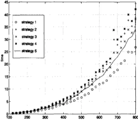
A n i m p o r t a n t d e t e r m i n a n t of p e r f o r m a n c e of t h e p e n a l t y a l g o r i t h m is t h e ini- t i a l i z a t i o n s t r a t e g y . T h i s consists in t h e choice of s u i t a b l e i n i t i a l values x ~ , yO a n d t o of x , y a n d t . A f t e r c o n s i d e r a b l e p r e l i m i n a r y e x p e r i m e n t a t i o n w i t h sev- 45
.I
40 o a~ete~1 + +~ x ~'mgy 3 9 20 ~+~+ o ~ 15 + . o~0
~
~176
j
oo 00 200 300 400 500 6G0 700 800Figure
5.1:Performance of initialization strategies for random nondegenerate problems
( ~ / . = 4).
eral a l t e r n a t i v e s , we h a v e set a s i d e t h e following s t r a t e g i e s as t h e m o s t p r o m i s i n g c a n d i d a t e s : STRATEGY 1 X o = 2 ( A T A ) - I A T b , yO = M I N R E S ( m / 2 , A x o _ b), t o = 0.01 • n • yO STRATEGY 2 x o = ( A T A ) - I A T b , yO = M I N R E S ( m / 2 , A x o _ b), t o = 0.1 • n • yO STRATEGY 3 x o = ( A T A ) - I A T b , yO = M I N R E S ( m / 2 , A x o _ b), t o = 0.01 • n • yO STRATEGY 4 x o = ( A T A ) - I A T b , yO = M I N R E S ( m / 4 , A x o _ b), t o = 0.1 • n • yO STRATEGY 5 x o = 2 ( A T A ) - I A T b , yO = M I N R E S ( m / 2 , A x ~ - b), t o = 0.1 x n x yO where M I N R E S ( k , r) r e t u r n s t h e k t h s m a l l e s t e n t r y of r in a b s o l u t e value. In F i g u r e 5.1, we i l l u s t r a t e t h e p e r f o r m a n c e of [INFS01_ u n d e r t h e s e five c o m p e t i n g
A PENALTY METHOD FOR LINEAR MINIMAX PROBLEMS 143
initialization strategies using randomly generated nondegenerate test problems with the ratio m / n = 4. The CPU time is given in seconds.
We observe that all five strategies perform similarly with a slight dominance of Strategy 1. As this test gave similar results for primal and dual degenerate problems we adopted Strategy 1 as our default initialization strategy for the randomly generated problems.
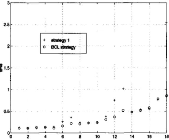
On the other hand, the performance of the above initialization strategies on the function approximation problems were somewhat inferior compared to the case of randomly generated problems. This is essentially due to the following observation. Although the optimal solution in these problems is nondegenerate the largest nonzero residuals at the solution can be as small as 10 -s . We refer to this property as near degeneracy. The performance o f / I N F S O / is affected negatively by this property as supported by the following theorem.
THEOREM 5.1. Let (x*,y*) be an optimal point for [LINFLP]. Let
~ , ~ 1 ifaVix * - y * = b i 01~(x ,y*) = ~ 0 otherwise, and Define
P =
[dx]
Let dz = du , ~ 1 i f a T x * + y * = b i 2,(x ,y*) = ( 0 otherwise. [ A T r i A T ATO2A --eTO1A + eT~)2A--AT(~le + AT~)2e ]
eT(~le + e T O 2 e J "be any solution to Pd = en+l and assume that (5.1) 0 1 ( - A d x +due) < 0, and 02(Ad~ +dye) > O.
Then, for 0 < t < to < 5, 0i(Mt) ---- ~1 and 02(Mr) = ~2 where 5 = min{51,52}
with 51 : maxr,(x.,y.)< 0 r l ( X * , y*) and 52 = minr~(x.,u*)>0 r2(x*, y*) .
The proof of this theorem can be obtained, mutatis mutandis, from the proof of Theorem 7 in [12]. A close inspection of conditions (5.1) reveals that they are equivalent to a nondegeneracy assumption which is satisfied by the function approximation problems. The theorem shows that one should expect to decrease the parameter t to the level of the smallest optimal nonzero residual value be- fore termination occurs. This implies that LINFSOL has to reduce t several times, resulting in a large number of iterations. This also makes the design of an effective starting strategy difficult for this class of problems. Bartels, Corm and Li [4] showed that the function approximation problems in the / ~ norm are characterized by a sign alternating property which states that at an optimal solution there are n + 1 equations whose residuals Ibi - aTxl correspond to the maximum residual t l A x - b Iloo with error terms (hi - a T x ) alternating in sign as the counter moves from 1 to n + 1. They propose an alternative starting point for their primal nondifferentiable penalty code based on Chebychev theory. In an
144 M U S T A F A C. P I N A R A N D S A M I R E L H E D H L I 3 2.5 2
~
1.5 1 0.5 0 0 § r~mti~y 1 o I~. ~m~r/ o @ 9 ~ 9 L i i i i 2 4 6 8 10 112 14 116Figure 5.2: Performance of initialization strategies for function approximation problems (problem number m = 50, 100, 200; n = 2, 3, 4, 5, 6, 7).
effort to improve the performance of LINFSOL on these problems we have exper- imented with several strategies based on the Bartels-Conn-Li recommendations. We have finally settled for the following strategy. Let zi = ~1 + n (~ - 1) for i = 1 , . . . , n + 1. Consider the (n + 1) • (n + 1) linear system of equations
n
f(zi)
-- ~__4"TjZ~ - 1 : ( - 1 ) i 0 , i : 1 , . . . , n + 1, j = lin the n + 1 unknowns 71,..-,7,~ and r We solve this system and use the solution as the initial point for LINFSOL. We choose t o = 10 - n + l following Theorem 5.1. This point results in a significant improvement in some problems. This is illustrated in Figure 5.2 where we compare the Bartels-Conn-Li strategy (BCL) with Strategy 1 described above using the exponential function over the interval [0, 1] (i.e., ~1 = 0 and ~2 = 1). We have used 18 problems where m assumes the values 50, 100 and 200, and n assumes the values 2 , 3 , 4 , 5 , 6 , 7 for each value of m in this order. This test was done on a SUN SPARC 4 Workstation.
5.4 Performance and comparison with the competing methods.
In this section we report the results of our comparisons with the Barrodale- Phillips code and the interior point algorithm of Zhang. We refer to the Barrodale- Phillips code as BP and to the predictor-corrector interior point code as P O P . To present our results we use eight plots where we report the average run time and iteration results for ten problem instances for given m and n. Our purpose is to display continuous behaviour as the problem size is increased. For the non- degenerate problems the first two plot reports run time and iteration results for problems where the ratio
m / n
is kept constant at two and m varies from 60 toA P E N A L T Y M E T H O D F O R L I N E A R M I N I M A X P R O B L E M S 145
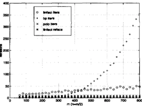
800 in steps of 20. To illustrate behaviour at a higher m / n ratio the next two plots report results where the ratio m / n is kept constant at four and m varies from 120 to 800 in steps of 20. For the primal and dual degenerate problems we give four plots (run time and iteration results) where we keep the ratio m / n = 2 and vary m from 60 to 800 in steps of 20. In the charts where iteration numbers are graphed BP iterations have been divided by 10 to make the plots easier to read. Furthermore, we also report the number of refactorizations in LINFSOL, in connection with the computations of factors L and D. All run time results are in CPU seconds exclusive of input and output. All three codes report results accurate to machine precision. We remark that LINFSOL may decrease the value of the parameter t to 10 -4 for some of the random problems.
S(m 2Sr 2 ~
1
15s t0~ 5C x •215 x ~ + + o o O O c ~ 8 6 o o o O 100 200 300 400 500 x ~ x - x . x x . x - x § § o o o o O o O o O O ~6OO 7O0 80O
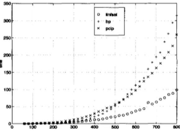
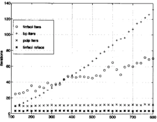
Figure 5.3: Run time comparison for nondegenerate problems (m/n = 2). We begin with the randomly generated nondegenerate problems with the ratio m / n = 2 in Figures 5.3 and 5.4. Here we observe that in general LINFSOL is increasingly faster than BP by a factor of three. It is also faster than PCIP by approximately a factor of two and a half. The number of iterations of LINFSOL grows very slowly while that of PCIP remains almost constant around 10. We observe a steady growth in the number of iterations of BP. LINFSOL performs between three and fourteen t-reductions on these problems in average. The average number of refactorizations remains around three.
In Figures 5.5 and 5.6 we present the same information for nondegenerate problems with the ratio m / n = 4.
We observe that LINFSOL outperforms both BP and PCIP by a factor of three and two and a half, respectively, as the problem size is increased. The number of t-reductions vary between five and sixteen. The average number of refactoriza- tions in LINFSOL is between three and four. PCIP uses between nine and eleven iterations on these problems.
In Figures 5.7, 5.8, 5.9 and 5.10 we report results on primal and dual degen- erate problems, respectively. Here, the ratio m / n is kept constant at two. The degree of primal degeneracy is pdeg = L-~-~] while we use ddeg = for dual
146 MUSTAFA C. P I N A R AND SAMIR ELHEDHLI 150
J
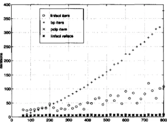
I O 0 00 0 IlrffllOI i t e m * b p i t e m x P e W n e t s i Iinfsol i ' e f a c s + + + _ o O o o o o O O O ~ ~ + ~ o o o ~ o o o o o o o o e ~ ~ 1 7 6 1 7 6 1 7 6 o O O + ~ ~ x x x x x x x x x x x x x x x x x x x x x x x x x x x x x x x x x x 1 ~ 2 ~ 300 4 ~ 500 600 7 ~ 800 m (n=nV2)Figure 5.4: Iteration comparison for nondegenerate problems ( m / n = 2).
70 6O 5 0 40 30 20 x X ~ + - x X i + x x § ! x x + o o < x + x 4 o 0 x x + o o ~ •215 § o x x x x X ~ p e ~ e e | 1 7 6
40O 500 6OO 700 8OO
Figure 5.5: Run time comparison for nondegenerate problems ( m / n = 4). degenerate problems.
We notice that LINFSOL performs better on primal degenerate problems com- pared to dual degenerate problems. This may be due to the fact that dual de- generate problems have non-unique primal optimal solutions. In our experience we have found this factor to weaken the performance of the penalty algorithm. It is worth mentioning here that the performance of BP is also adversely affected by dual degeneracy. For both classes we observe that LINFSOL becomes increas- ingly faster than BP. More precisely, for primal degenerate problems EINFSOL sustains a speed-up of three and a half over BP while it reaches a speed-up of three in the dual degenerate case. For primal degenerate problems LINFSO[ is twice as fast as PCIP. On dual degenerate problems, PCIP appears to do better than IINFSOL reaching a speed-up factor of one and a half. This is reflected in the number of iterations of PCIP, which rarely exceeds six for dual degenerate problems while it is around eleven in average for primal degenerate test cases.
A P E N A L T Y M E T H O D F O R L I N E A R M I N I M A X P R O B L E M S 1 4 7 140 "F ~ T "1 r 120 + 100 | BO o o o ~ ~ o O o ~ ~ + 2o + + + ~ * X X X X X X X X X X X X X X X X X X X X X X X X X X X X X X X X : ~ " i i + § 1 8 4 x po40 ~ml + + o + + ~ o + o O o ~ o o + | o
Figure 5.6: Iteration comparison for nondegenerate problems ( m / n = 4).
40~ 3O0 2 ~ 15{] IOQ 5Q x . x x - x X x x . ~ x o o ~ X X X o o o o O O ~ 1 7 6 ~ x x o O o . . . . ~ c 9 ~ 1 7 6 1 7 6 1 7 6
Figure 5.7: Run time comparison for primal degenerate problems ( m / n = 2).
The number of t-reductions of LINFSOL for the dual degenerate case varies be- tween 1 and 28 while it is between two and eight for the primal degenerate case. The number of refactorizations is between four and nine for the dual degenerate case whereas it remains constant around two for the primal degenerate case.
We can infer the following conclusions from the above results.
9 The penalty method appears to do best on nondegenerate and primal de- generate problems.
9 The penalty method is expected to perform better after a certain threshold problem size is reached.
9 In all cases, we have observed that the number of refactorizations of the penalty method remains almost constant as the problems become larger. * The iteration charts reveal that the simplex method has a steady growth
148 MUSTAFA C. PINAR AND SAMIR ELHEDHLI 40c 35~ 3Gc 25c 15C 10C 5C I" ~ ' ~ "
I~
~
i
i+
+ + + + i + + + + - + + + :i
"
100 2 0 0 3 0 0 4 0 0 5 0 0 eGO 7 0 0 8 0 0 m ( n , . m ' 2 )Figure 5.8: Iteration comparison for primal degenerate problems ( m / n = 2).
5OO 45O 4 ~ 38O 3 ( ~ 1 ~ - o + ~ , * O o o ~ x x x +.* o ~ x • x~ - ,==- . . . , , , i ~ ; ~ " ~ ~ t ~ 2 0 0 3 0 0 4 0 0 5 0 0 6 0 0 7 ~ 8 0 0
Figure 5.9: Run time comparison for dual degenerate problems ( m / n = 2).
in the number of iterations. The interior point method uses an almost constant number of iterations for a given problem class while the penalty method exhibits a very low growth rate in the number of iterations as the problem size is increased.
9 The predictor-corrector algorithm seems to do best on dual degenerate problems.
Finally, we summarize our experience with function approximation problems. For this purpose we choose to approximate the exponential, the square root and the sine functions on the interval [0, 1]. We have solved 54 problems of varying dimensions altogether, 18 for each function. These experiments showed that
B P is about ten times faster than both L I N F S O L and P O P on the average while LINFSOL and POP exhibit a similar performance. Two factors play an important role here. The first one is the outstanding performance of BP on these problems.
A P E N A L T Y M E T H O D F O R L I N E A R M I N I M A X P R O B L E M S 149 400 , , § bp Item
I
26C 1,5C 10C 5C + + i + * + 4 § O . ' " o o o c ~ o o 0 + + ~ 1 7 6 o o o o o ~ § b o Oo o ' o o O o 0 ~ ~ ~ 9 o ~ o mik~mMmm n m x i : 1 1 ~ m N i N m # m m m ~ m m N | m # m m m N N m ~ 100 200 $00 4(X) ,500 600 700 800Figure 5.10: Iteration comparison for dual degenerate problems (m/n = 2 ) .
This is partially due to the fact these problems have at most eight variables. This is a range where BP is very efficient. Furthermore, Bartels, Corm and Li [4] prove that the high efficiency of the BP algorithm on function approximation problems is due to the fact that BP exploits the special structure of function approximation problems. It is proved in [4] that after the first stage (Phase I) BP finds a feasible solution that satisfies the sign alternating property as described in Section 5.3. The second factor is that the optimal solution is usually near degenerate for these problems as defined in Section 5.3. This degrades the performance of LINFSOL considerably. We substantiated this observation by Theorem 5.1 in Section 5.3. We would like to note, however, that the accuracy of the solution is maintained in all the cases, and LINFSOL solves all these problems within at most three CPU seconds. Interestingly, the performance of P a P deteriorates considerably on these problems as well. A similar degradation in performance with function approximation problems is reported in [9] for the exact penalty method and is attributed to near degeneracy as well.
6 Conclusions.
In this paper, a penalty continuation algorithm was designed for linear for problems. The computational results indicate that the algorithm is stable and accurate on different kinds of problems. Furthermore, it was shown to suc- cessfully compete with Barrodale-Phillips algorithm and the predictor-corrector primal-dual interior point algorithm of Zhang on a wide range of random prob- lems. Based on our tests, the algorithm seems to perform best on problems with no special structure (e.g., problems not derived from function approximation) where the number of variables exceeds a certain threshold.
Acknowledgement.
The assistance of the associate editor K. Madsen, and the careful reviews of two anonymous referees are gratefully acknowledged.
1 5 0 MUSTAFA C. PINAR AND SAMIR ELHEDHLI
R E F E R E N C E S
1. R. H. Bartels and G. H. Golub, Stable numerical methods/or obtaining the Cheby-
shev solution to an overdetermined system of equations, Comm. ACM., 11 (1968),
pp. 401-406.
2. I. Barrodale and C. Phillips, An improved algorithm for discrete Chebychev lin-
ear approximation, in Proc. Fourth Manitoba Conf. on Numerical Mathematics,
University of Manitoba, Winnipeg, Canada, 1974, pp. 177-190.
3. R.H. Bartels, A. R. Corm, and C. Charambous, On Cline's direct method for solving
overdetermined linear systems in the ~oo sense, SIAM J. Numer. Anal., 15 (1978),
pp. 225-270.
4. R. H. Baxtels, A. R. Conn, and Y. Li, Primal methods are better than dual methods
for solving overdetermined linear systems in the goo sense?, SIAM J. Numer. Anal.,
26 (1989), pp. 693-726.
5. D. P. Bertsekas, Newton's method for linear optimal control problems, in Proc. of Symposium on Large Scale Systems, Udine, Italy, 1976, pp. 353-359.
6. T. F. Coleman and Y. Li, A global and quadratically convergent method for linear
~ problems, SIAM J. Numer. Anal., 29 (1992), pp. 1166-1186.
7. J. Dongarra, J. Du Croz, S. Hammarling, and R. Hansen, An extended set of basic
linear algebra subprograms, ACM Trans. Math. Software, 14 (1988), pp. 1-17.
8. R. Fletcher, Practical Methods of Optimization, Second Edition, John Wiley & Sons, Chichester, 1987.
9. B. Joe and R. Bartels, An exact penalty method for constrained, dicrete, linear too
data fitting, SIAM J. Sci. Comput., 4 (1983), pp. 69-84.
10. K. Madsen and H. B. Nielsen, Finite algorithms for robust linear regression, BIT, 30 (1990), pp. 682-699.
11. K. Madsen and H. B. Nielsen, A finite smoothing algorithm for linear gl estimation,
SIAM J. Optim., 3 (1993), pp. 223-235.
12. K. Madsen, H. B. Nielsen, and M.~. Pmar, New characterizations of ~1 solutions
of overdetermined linear systems, Oper. Res. Letters, 16 (1994), pp. 159-166.
13. K. Madsen, H. B. Nielsen, and M.~. Plnar, A new finite continuation algorithm
for linear programming, SIAM J. Optim., 6 (1996), pp. 600-616.
14. NAG Fortran Library Routine Document, Numerical Analysis Group, 1981. 15. H. B. Nielsen, AAFAC: A Package of Fortran 77 Subprograms for Solving AT Ax =
c, Report NI-90-11, Institute for Numerical Analysis, Technical University of Den- mark, 1990.
16. M. ~. Plnar, Piecewise linear pathways to the optimal solution set in linear pro-
gramming, J. Optim. Theory Appl., 93 (1997), pp. 619-634.
17. S. A. Ruzinsky and E. T. Olsen, gl and ~ minimization via a variant of Kar-
markar's algorithm, IEEE Transactions on Acoustics, Speech and Signal Processing,
37 (1989), pp. 245-253.
18. G. A. Watson, Approximation Theory and Numerical Methods. John Wiley, New York, 1980.
19. Y. Zhang, Primal-dual interior point approach for computing the gl -solutions and
~cr -solutions of overdetermined linear systems, J. Optim. Theory Appl., 77 (1993),