Optimum feedback patterns in multivariable control systems

(1)

Optimum feedback patterns in multivariable control systems

KONURALP

U N Y E L ~ O C L U ~

and M. EROL SEZER?

The following problem is considered: 'Given a multivariable system with nl inputs and r outputs and an r x nl matrix whose non-negative (i,j)th element represents the

cost of setting LIP a feedback link from the,jth output to the ith input, find a set of feedback links with minimum total cost, which does not give rise to fixed modes'. Utilizing the graph-theoretic churiicterization of structurally fixed modes, the problem is decomposed into two subproblems. which are then solved by using concepts and results from network theory. A combination of the optimum solutions of the subproblems provides a suboptimal solution to the original problem.

1. Introduction

Consider a linear multivariable system described by

where . Y E R", 11 E R'", and y~ Rr denote the states, inputs, and outputs of .'Y'

respectively. Suppose that each output/input pair (yj. u i ) is associated with a non- negative number

kb

which represents the cost of setting up a feedback path from output yj to input u i . The problem we consider is to identify a set of feedback paths with minimum total cost, which allows for a satisfactory control of .'f using dynamic feedback controllers in these paths. I t is well known ( Wang and Davison 1973, Sezer and Siljak 198 1, Reinschke 1984) that a satisfactory control can be achieved using dynamic compensators that obey a given feedback structure constraint if the system has rlo fixed modes with respect to the given feedback structure. Thus the problem is to identify the cheapest feedback pattern that avoids fixed modes.

Although several characterizations of fixed modes exist in the literature (Corfmat and Morse 1976, Anderson and Clements 198 1 ) including graphical ones related to structurally fixed modes (Pichai ut al. 1984, Reinschke 1984), they are not directly applicable to the problem considered here, simply because testing of all possible feedback patterns for feasibility requires enormous computations. In the present work, we formulate the problem in a structural framework to avoid the difficulties involved in algebraic tests, and propose a reasonable sequential solution procedure through a decomposition of the problem based on a classification of structural fixed modes. We show that the two subproblems obtained by decomposition can be reformulated as network flow problems (Bazaraa and Jarvis 1977, Chaera er al. 1977), which can be solved using adaptations of known algorithms.

Matrices and vectors are denoted throughout by upper and lower case italic letters; binary matrices by upper case boldface letters; and abstract objects such as a

Received 25 January 1988. Revised 28 April 1988.

t Electrical and Electronics Engineering Department, Bilkent University, P.O. Box 8,

Ankara 06572, Turkey.

(2)

792 K. ~ n ~ e l i o g l u and M. E. Sezer

set, a system etc. by script letters. A superscript c indicates the cost associated with a matrix or its elements.

2. Digraphs, system structure, fixed modes

In this section we review some basic concepts from graph theory (Harary et al. 1965, Deo 1974) and the structural representation of dynamical systems through digraphs (Coates 1959, Siljak 1978), and results concerning fixed modes in multivariable systems (Wang and Davison 1973), and the graphical characterization of structurally fixed modes (Pichai et al. 1984).

A digraph 9 = ( V , &) is an ordered pair, where V is a finite set of vertices, and 8 is a finite set of ordered pairs of vertices called edges. If (vj, vi) E 8, then the vertex vj is said to be adjacent to the vertex vi. An adjacency relation defines a binary matrix

M = (mij), called the adjacency matrix of 9 , such that mij = 1 if and only if (vj, vi) E 8.

A digraph is completely characterized by its adjacency matrix. A sequence of edges ((vl, vZ), (vZ, v3),

.

. .

, (v, - 0,)) where all vertices are distinct, is called a path from v, to

v, . In this case, u, is said to be reachable from 0,. If v, coincides with v,, then the path is called a cycle. Any two vertices which are mutually reachable are said to be strongly connected. A maximal subgraph containing strongly connected vertices is called a strong component of

9.

Strong components are uniquely determined. Reachability relation too can be described by a binary matrix R = (rij) such that rij = 1 if and only if vj reaches vi.

The structure of the system 9 in (1) can be conveniently described by a binary matrix

called the system structure matrix, where A = (aij) with a i j = 1 if and only if aij # 0, and B and C are defined similarly. The digraph 9 which assumes S as its adjacency matrix is called the digraph of the system 9'. For convenience, the vertex set of 9 can be partitioned as Y" = 9" u4P u g , where 3, +Y, and Oy denote the sets of state, input, and output vertices.

Two systems which have the same system digraph are called structurally equivalent. System structure matrices of structurally equivalent systems are related by permutation transformations. Structurally equivalent systems form an equivalence class. A property is said to be a structural property of a system if it holds for at least one member of the equivalence class to which that particular system belongs.

Let K = (kij) be an m x r binary matrix, which specifies a feedback pattern for the system 9'in (1) such that kij = 1 if and only if a feedback from output yj to input ui is allowed. Let K be a constant matrix in the equivalence class K. Then, the closed-loop system consisting of 9 and the feedback law

where v E

Rm

stands for reference inputs, is represented by the closed-loop system structure matrix

(3)

Optimum feedback patterns in multivariable control systems 793

Accordingly, the closed-loop system digraph becomes = (-Y, &ugK), where

gx = { ( y j , u i ) : k i j = 1) contains the feedback edges.

The set of fixed modes of 9' with respect to K is defined as A,=

r )

A(A+ BKC)

K E K

where A( ) denotes the set of eigenvalues of the indicated matrix. It is known that all the poles of 9'can be assigned arbitrarily using dynamic feedback compensators that obey the feedback structure constraint specified by some K if and only if A, = 0 , that is, 9' has no fixed modes with respect to K.

Fixed modes of a system originate either from a perfect matching of the numerical values of the system parameters, or from the special structures of the system and the feedback pattern. In the latter case, all systems in the same equivalence class have fixed modes, and the system is said to have structurally fixed modes. Structurally fixed modes can be characterized in terms of the closed-loop system digraphs as stated by the following lemma.

Lemma 1 (Pichai et al. 1984)

A structured system S has no structurally fixed modes with respect to a feedback pattern K if and only if the following two conditions are satisfied:

(a) the closed-loop system digraph

@

is covered by a collection of vertex disjoint cycles;

(b) each state vertex of occurs in a strong component that contains a feedback edge.

If 9'has no structurally fixed modes with respect t o K we describe this fact symbolically as A, =

0.

The state vertices that violate condition (b) of Lemma 1 correspond to a principal submatrix of A in 9. The modes of the associated structured subsystem are defined as B-type structurally fixed modes of 9'.Consider the subgraph obtained from

d

by removing these state vertices and the edges connected to them. If this subgraph has any structurally fixed modes, they are due to violation of condition (a), and are therefore called A-type structurally fixed modes of 9'. Note that A-type structurally fixed modes are always at the origin, and cannot be associated with a part of 9'. This way, structurally fixed modes of a system can be classified into two distinct groups, both of which result from an insufficient interconnection among system variables. This classification of fixed modes is useful in decomposing the optimization problem formulated in the next section.

3. Problem statement and decomposition

The problem we consider is pole placement in a system

9 '

using minimum cost dynamic feedback compensators. For this purpose we define the total cost of a given feedback pattern K to be

and formulate our problem

min c( K)

9:

(4)

794

K.

~ n ~ r l i o f l u und

M .

c(Ki) ( 10) where K O is the optimal solution of the original problem

9.

From (10) it follows that

that is, the solution Kkbtained through a decomposition of 9 is at most 100% more costly than the optimum solution. We can, therefore, think of K 9 s a suboptimal solution of problem 9 .

We note that once an optimal solution to one of the above problems is obtained, then some of the feedback links that appear in the corresponding feedback pattern may help satisfy the feasibility condition of the other problem without any additional cost. This suggests a sequential optimization procedure, where the two problems are solved sequentially with the cost matrix modified after solving the first problem. Thus, with K: =

(ky)

being a solution of problem PA, we modify the cost matrix K c into K > = (kij'), where

0,

ky=

1

k;; =

kij, otherwise and replace problem 9', with

min cA(K) ~ A B :

(5)

Optimum .fhedhuck putterns in multivuriuhle control systems 795 where

Now, with K:, being the optimum solution of problem q A B , we have

Thus, defining the suboptimal solution obtained through the sequential optimization of the problems YA and PAB as

we have

which shows that the loss due to decomposition is decreased by employing a sequential optimization scheme.

Obviously, one could interchange the order of the two problems, and start with YB instead. In this case, problem .PA would be replaced by

min cB(K)

~ B A

s.t. A:=@

I

where K', and cB(K) are similar to Kc, and cA(K), and are defined after a solution Kg to problem PB is obtained. In what follows, we drop the two-letter subscript notation for convenience, with the understanding that PB denotes the modified problem PA, in the sequence ( g A , 9,) and 9, denotes PBA in the sequence (9,, PBA). We also employ the notation P A ( 9 , K c ) or P B ( 9 , Kc) to indicate explicitly the digraph and the cost matrix upon which PA or PB is formulated.

Before considering solution procedures for PA and P B , we would like to point out that, in general, the ultimate suboptimal solution depends on the order in which the two subproblems are solved as we demonstrate with an example in

5

7.

4. Solution of problem P A ( 9 , Kc)

It is known (Pichai et al. 1984) that condition (a) in the statement of Lemma 1 is equivalent to

where gr (.) denotes the generic rank of the indicated matrix, and is equal to the maximum number of non-zero .entries that lie on different rows and columns (e.g. Shields and Pearson 1976, Duff 1981). Therefore, an alternative statement of problem

PA can be given as

min c(K)

PA :

s.t. g r ( S ) = n + m + r

I

.

In this formulation the constraint is stated in terms of the closed-loop system structure matrix S , but the cost involves only a part of

S,

namely K. In order to translate the

(6)

796 K . ~ n ~ e l i o g l u and M . E. Sezer

cost into one involving S , we define the system cost matrix

SC

as

where A' = (a:,) with

B' and C' are defined similarly;

I"

is a matrix of suitable dimension, consisting of all y; and I' has zero diagonals and y off-diagonals. In other words,

S'

is obtained from

S

by replacing zero elements by y and non-zero elements by 0 except those of K, which are replaced by the corresponding costs. Now defining the total cost associated with a system structure matrix

S

to be

we reformulate problem PA as

min c(S) gA :

s.t. g r ( S ) = n + m + r

1

Problem 9A as stated in (23) is known as the 'assignment problem', which is equivalent to a linear network flow problem (Bazaraa and Jarvis 1977, Chaera et al. 1977). An efficient solution procedure for the assignment problem is the Hungarian assignment algorithm, which is repeated below for convenience.

Hungarian assignment algorithm (Bazaraa and Jarvis 1977, Kuhn 1955)

Step 1. For each row of

S',

subtract the minimum element of the row from all the elements of the row.

Step 2. Repeat Step 1 for columns of

9'.

Step 3. Pick the maximum number of zeros in

9'

which lie on different rows and columns. If a zero is picked from every row, go to Step 5.

Step 4. Draw a minimum number of lines (vertical or horizontal) that cover all zeros in

3'

(the number of lines is the same as the number of zeros picked in Step 3). Find the minimum of all elements which are not covered by these lines; subtract the minimum from the uncovered elements and add to the ones that are covered by both horizontal and vertical lines. G o to Step 3.

Step 5. The optimum solution of problem PA is obtained simply by setting 1, if a zero at the corresponding position of K c is picked kp: =

0, otherwise

Before closing the section, we would like to point out. that Step 3 of the Hungarian assignment problem is the maximum transversality problem (Duff 1981), and is equivalent to computing the generic rank of a matrix.

(7)

Optimum feedback patterns in multivariable control systems 797 5. Solution of problem P B ( 9 , Kc)

Considering condition (b) of Lemma 1, we note that if a state vertex xi occurs in a strong component of the closed-loop system digraph

&

which contains a feedback edge, then all state vertices that are strongly connected to xi in the open-loop system digraph

9

have the same property. Therefore, a condensation of the strong components of 9 before inserting the feedback edges does not effect the set of feasible feedback patterns for problem PB. In other words, P B ( 9 , Kc) is equivalent to PB(9*, Kc), where 9* is obtained from 9 by condensing the strong components. Let the state vertices of 9 * be %* = {xf, x f ,

. ..,

x;). Then, condition (b) requires that each x r in

a*

reaches itself through a path (which should necessarily include a feedback edge, as 9 * is acyclic). This observation allows us to reformulate condition (b) as a generalized assignment problem on a block cost matrix

where each block

mpq

= (G~9),x, of W is associated with a pair of state vertices (x:, x;), and has the elements

{kc, if ui reaches xz and x: reaches yj in 9 * Gpg =

" , otherwise

In other words, GGq is the cost of a path from x8 to x,* through yj and ui, which is infinity if no such path exists. It is clear that condition (b) is equivalent to picking N elements in @, which are located in different block rows and columns of

w.

Now, .PB can be reformulated as min c(K) PB : s t . block gr (KG) = N where block gr (KG) = block gr

(w)

= gr (W) ₍₂₇₎ with W = (w,,),

.

defined as

1, ifG5q#y for some(i,j)

W ~ 4 =

0, otherwise

We note that the generalized assignment problem in (26) is actually a network flow problem involving the transportation of supplies at the state vertices to themselves over the feedback edges. However, it is different than the ordinary assignment problem in (23) in that if the same feedback edge is picked more than once in different block rows and columns of to satisfy the feasibility condition, no extra cost is charged for the additional choices. Because of this, PB in (26) is a non-convex, non- linear problem, which cannot be solved by linear algorithms. In the following, we present an implicit enumeration algorithm for the solution of PB. For this purpose we first introduce the following notation.

798 K. ~ n ~ e l i o g l u and M. E. S u e r

Here J(1) = 1 or 0 means the corresponding feedback edge el is or is not included in the current pattern; J(1) = F indicates that el may later be included in the pattern, i.e. el is free; and finally J(1) = U means addition of el results in a feedback pattern whose cost is no smaller than the current optimum, i.e. el is useless at that step. The cost of a feedback pattern described by the current form of J is denoted by c(J), and is computed as

Finally, the current minimum is denoted by c*, and the current best pattern by J*. Implicit enumeration algorithm

Step 1. Step 2. Step 3. Step 4. Step 5. Step 6. Step 7. Initialization. Set J(1) = F, I S 1 S s, c* = y, k: = 1, 1

<

i

<

m, 1

<

j

<

1. Find L = min (I: J(1) = F ) . Set J ( L ) = 1.

Check J for feasibility (subroutine). If J is feasible, set J

*

= J , c* = c(J), and go to Step 6. Otherwise proceed to the next step.

For 1

<

1

<

s and J(1) = F, if c ( J )

+

c, 2 c*, set J(1) = U. If there remains any 1

with J(1) = F proceed to the next step. Otherwise go to Step 6.

Check J for potential feasibility (subroutine). If J is potentially feasible, go to Step 2. Otherwise proceed to the next step.

If J(1) # 1 for all I

<

1

<

s, proceed to the next step. Otherwise, find L = max {L: J(1) = I), set J(L) = 0, J(1) = F for I > L, and go to Step 4. For 1

<

I < s and J*(1) # 1, find the unique pair of indices (i, j) defined by I, and set k v = 0; KOB = ( k v ) is an optimum solution of YB.

Subroutine for feasibility and potential feasibility

Step 1. Construct W = (w,,),

.

,

corresponding to J as follows: (a) initially w,, = 0, 1 d p, q

<

N;

F). The algorithm is a depth-first search (Tarjan 1972) on the tree, where a branch is bounded when either the pattern corresponding to its root is a feasible one with a smaller cost, or all the subsequent patterns are infeasible or have higher costs. .

We note that the proposed implicit enumeration algorithm can be improved considerably if more attention is paid to the choice of the feedback edge to be included

and a modified cost matrix K', such that optimum solutions of P B ( 9 * , Kc) and q A ( g M , K',) are the same. The idea is motivated by the fact that if a set of feasible solutions to P B ( 9 * , Kc) which contains the optimum solution

KE

were known, then one could always and easily construct 9, and K', such that PA(9,, K',) admits Kg as optimum solution. In the following, we show that for a class of digraphs 9 * , P A ( g M ,

Kh)

can be constructed without knowing the optimum solution

We start by defining the index sets I , and J, associated with the state vertices of 9 * as

I , = {i: ui reaches x: in B*), J, = { j: x: reaches yj in 9*), 1 = 1,2,

...,

N Suppose that there exists a permutation (I,, l,,

...,

1,) of the state vertices X * of 9 * such that

Considering the reachability matrix

(10)

800 K . ~ n ~ e l i o g l u and M . E. Sezer

matrices P,, P,, and P, such that P:G*P, and P,H *Px have the following structures.

where

1

indicates that the region is filled with 1s. Let the sets of input and output vertices of 9* be partitioned in accordance with the structures of P:G*P, and P,H*P, as

We now construct an intermediate digraph 9:= (XT u

@T

u gf,

QT),

which is characterized by the adjacency matrix

(11)

Optimum feedback patterns in multivariable control systems

Note that the state vertices of 23: are arranged in the form of a chain, each group of inputs of 9 * belonging to the same input set @, is replaced by a single input u:, and similarly each group of output vertices belonging to the same output set tY, is replaced by a single output y,* in 23:.

We further define a modified cost matrix as K & =

( k i y ) ,

.

,, where min {k;,: ui E +?,, gj E g,), if s, d t,

7, otherwise

It is now easy to see that to any optimal solution of YB(9*, Kc) there corresponds an optimal solution of P B ( 9 ? , K',) with the same cost and vice versa, so that the original problem g B ( 9 * , Kc) can be replaced by pB(9;, K',). At this point it should be noted that gB(9:, K',) is already much simpler than YB(9*, Kc) because of the special structure of

97

and the fact that K', contains fewer non-y entries than K c does (which speeds up Steps 4 and 5 of the implicit enumeration algorithm).

The next step is to construct gM from 9; such that optimum solutions of PB(9T, K',) and P A ( g M , K',) coincide. For this purpose, we first note the following:

(a) each feedback edge (y:, u:), s, ,< t,, defines a unique cycle in the closed-loop digraph

a:,

which covers the state vertices x f , s, d i

<

t,;

( h ) a given feedback pattern is feasible for 9 B ( 9 f , K',) if and only if the family of cycles defined by the corresponding feedback edges cover all the state vertices; (c) a state vertex can be common to at most two cycles in a cycle family defined by

an optimal feedback pattern.

Hence, PB(Q,*, K',) is also a state vertex covering problem. However, unlike problem 9,, the cycles that cover the state vertices of B f need not be disjoint. This difficulty can be overcome, by expanding the state vertices of 9: as explained below.

(12)

802 K . ~ n ~ r l i o ~ l u and M . E. Sezrr

M

k . . = in.1 2, otherwise 3, if i = t , for some 1

<

q

<

R - 2 2, otherwise

The modified digraph 9, = (TM u&* u

Y*,

gM) is then described by the adjacency matrix

SM =

CM 0 I R

where AM = ( A t ) ,

.

,, whose blocks are defined as follows:

where the indicated rows and columns need not exist if xT or x:+, has no inputs and/or outputs connected to them. Finally,

and

B M

and

C M

are similar to

B,*

and Cf with dimensions modified as necessary. With

9,

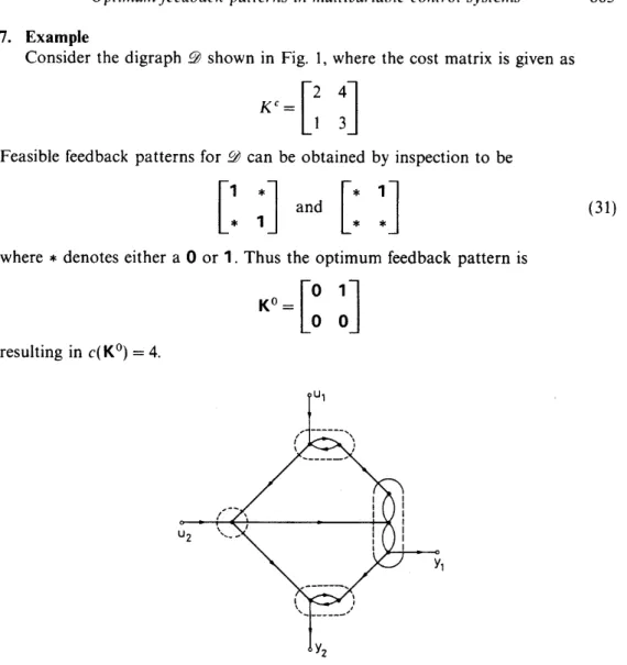
defined as above, it is a straightforward but a tedious task to show that to any non-redundant feasible solution of PB(9F, K',) there corresponds a feasible solution of P A ( g M , K h ) containing exactly the same feedback edges, and vice versa. The steps involved in the construction of g M are explained by an example in the next section.

(13)

Optimum feedback patterns in multivariable control systems 803 7. Example

Consider the digraph 9 shown in Fig. 1, where the cost matrix is given as

Feasible feedback patterns for 3 can be obtained by inspection to be

where

* denotes either a

0 o r I . Thus the optimum feedback pattern is

resulting in c ( K O ) = 4.

Figure 1 . Digraph considered in the example.

Now consider a decomposition of Y ( 9 , K c ) into Y A ( 9 , K C ) and P B ( 9 , K c ) . The optimum solution of Y A ( 9 , K c ) is obtained directly by applying the Hungarian assignment algorithm to

Sc

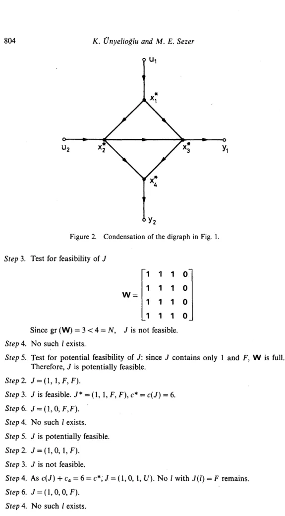
as

To illustrate the solution of Y B ( 9 , K c ) , we first form the digraph 9 * shown in Fig. 2, by condensing the strong components of

9,

and rename the feedback edges as

( k l l , kl2, k21, k22) = ( e l , e2, e3, e.4) The implicit enumeration algorithm proceeds as follows. Step 1 . J = ( F , F, F, F ) , c* = y.

(14)

K . ~ n ~ e l i o g l u and M . E. Sezer

Figure 2. Condensation of the digraph in Fig. 1. S t e p 3. Test for feasibility of J

Since gr ( W ) = 3 < 4 = N , J is not feasible. S t e p 4. No such 1 exists.

S t e p 5. Test for potential feasibility of J : since J contains only 1 and F , W is full. Therefore, J is potentially feasible.

S t e p 2 . J = ( l , 1, F , F ) . S t e p 3. J is feasible. J * = ( I , 1 , F , F ) , c* = c ( J ) = 6 . S t e p 6 . J = ( l , O , F , F ) . S t e p 4. No such 1 exists. S t e p 5. J is potentially feasible. S t e p 2 . J = ( 1 , 0 , 1, F ) . S t e p 3. J is not feasible. S t e p 4. As c ( J )

+

c , = 6 = c*, J: = ( 1 , 0 , 1, U ) . No I with J ( I ) = F remains. S t e p 6. J = ( l , 0 , O , F ) . S t e p 4. No such I exists.

(15)

Optimum feedback patterns in multivariable control systems 805 Step 5. J is potentially feasible.

Step 2. J = ( l , 0 , 0 , 1).

Step 3. J is feasible. J

*

= ( 1,0,0, I), c* = c ( J ) = 5.

Step 4. No such I exists. No 1 with J ( 1 ) = F remains. Step 6. J = (0, F, F, F).

Step 4. No such I exists. Step 5. J is potentially feasible. Step 2. J . = (0, 1, F, F).

Step 3. J is feasible. J * = (0, 1, F, F), c* = c(J) = 4. Step 6. J = (O,O, F, F).

Step 4. No such 1 exists.

Step 5. J is not potentially feasible. Step 6. J(1) # 1 for all I.

Step 7.

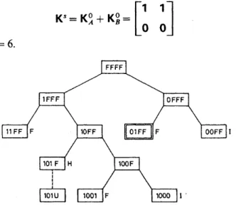
The tree generated by the implicit enumeration algorithm is shown in Fig. 3, where the branches are terminated at the nodes marked as F, H, or I. An F indicates that the corresponding pattern is a feasible one better than the previous feasible one, an H marks a pattern whose cost is higher than the cost of the current best pattern (even if it is potentially feasible), and an I marks the infeasible patterns.

The suboptimal solution to problem 9(9, K c ) is obtained by combining K! and K i as

resulting in c(Ks) = 6 .

OOFF I

(16)

806 K . ~ n ~ r l i o f l u und M . E. Sezer

Now considering the reachability matrix of 9 * , we observe that

which already have the special forms in (31), with s, = 1, s2 = 2; t, = 3, t2 = 4. The intermediate digraph

9 7

is shown in Fig. 4, and K ', = K

'.

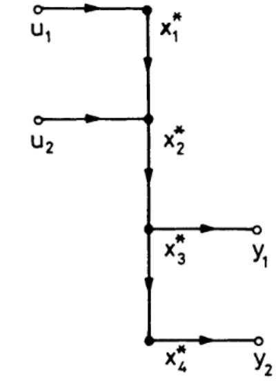
It can easily be verified that application of the implicit enumeration algorithm to YB(9T, KC,) yields the same optimal feedback pattern Kg.

To illustrate the construction of 9,, we compute

and expand xT and x: as shown in Fig. 5. Application of the Hungarian assign-

Figure 4. Intermediate digraph corresponding to the digraph of Fig. 2.

(17)

Optimum fkedback patterns in multivariable control systems 807

ment algorithm to the modified system cost matrix

Sh

yields the same optimum solution KE.

If we employ the sequential optimization procedure, the cost matrix Kc is modified to

after solving p A ( g , Kc). Now, the optimum solution of g B ( 9 , K',) is obtained, either by the implicit enumeration algorithm .or through the use of the modified digraph, to be

The corresponding suboptimal solution will then be

resulting in c(K",) = 5.

Finally, we point out that if the sequential optimization procedure is employed in the sequence (PB, PA), then we obtain

so that K", = KO, that is the suboptimal solution coincides with the optimal one.

8. Conclusions

The problem of identifying a minimum cost feedback pattern, which does not give rise to structurally fixed modes, is considered. The problem is formulated in a graph- theoretic setting, and the graphical characterization of the fixed modes is utilized as the basic tool. A classification of the structurally fixed modes into two distinct types allows for a decomposition of the problem into two simpler subproblems, whose optimum solutions can be combined to obtain a suboptimal solution to the original problem. These two subproblems are reformulated as network flow problems, and concepts from network theory are utilized to obtain their solutions.

Several remarks can be made concerning the formulation and the solution of the problem. First, it is observed that the problem of choosing a feasible feedback pattern that includes a minimum number of feedback edges, which was considered previously by Sezer (1983), is a special case of the problem formulated in this work, which corresponds to the case ktj = 1 for all i, j for which ktj # y. However still more general formulations are possible. For example, fixed initial costs can be assigned to the inputs and outputs in addition to the feedback costs. It may also be meaningful to group the inputs and outputs as in decentralized control, and assign costs to the multiple feedback links among the groups rather than to the individual links. These complications, however, make the already non-linear problem even more difficult to handle.

(18)

808 Optimum feedback patterns in multivariable control systems

REFERENCES

ANDERSON, B. D. O., and CLEMENTS, D. J., 1981, Automatica, 17, 703.

BAZARAA, M. S., and JARVIS, J. J., 1977, Linear Programming and Network Flows (New York: Wiley).

CHAERA, V., MOORE, J., and GHARE, P. M., 1977, Applications of Graph Theory Algorithms (New York: North-Holland).

COATES, C. L., 1959, I.R.E. Trans. Circuit Theory, 6, 170. CORFMAT, J. F., and MORSE, A. S., 1976, Automatica, 11, 479.

DEO, N., 1974, Graph Theory with Applications to Engineering and Computer Science (Englewood Cliffs, N.J.: Prentice-Hall).

DUFF, I. S., 1981, Assoc. Comput. Machinery. Trans. Math. Software, 7, 315.

GARFINKEL, R., and NEMHAUSER, G., 1972, Integer Programming (New York: Wiley).

HARARY, F., NORMAN, R. Z., and CARTWRIGHT, D., 1965, Structural Models: An Introduction to the Theory of Directed Graphs (New York: Wiley).

KUHN, H. W., 1955, Naval Res. Log. Quart., 2, 83.

PICHAI, V., SEZER, M. E., and SILJAK, D. D., 1984, Automatica, 20, 247. REINSCHKE, K., 1984, Int. J. Control, 39, 71 5.

SEZER, M. E., 1983, Minimal essential feedback patterns for pole assignment using dynamic compensation. Proc. 22nd I.E.E.E. Conf on Decision and Control, San Antonio, Texas, pp. 28-32.

SEZER, M. E., and SILJAK, D. D., 1981, Systems Control Lett., 1, 60. SHIELDS and PEARSON, 1976, I.E.E.E. Trans. autom. Control, 21, 203.

SILJAK, D. D., 1978, Large-scale Dynamic Systems: Stability and Structure (New York: North- Holland).

TARJAN, R., 1972, SlAM J. Comput., 1, 146.