Investigation of the low temperature dynamics of a modified toric code

INVESTIGATION OF THE LOW

TEMPERATURE DYNAMICS OF A

MODIFIED TORIC CODE

a thesis submitted to

the graduate school of engineering and science

of bilkent university

in partial fulfillment of the requirements for

the degree of

master of science

in

physics

By

Noor Al Huda Yousuf

August 2020

Investigation of the Low Temperature Dynamics of a Modified Toric Code

By Noor Al Huda Yousuf August 2020

We certify that we have read this thesis and that in our opinion it is fully adequate, in scope and in quality, as a thesis for the degree of Master of Science.

Cemal Yalabık(Advisor)

Bilal Tanatar

S¸inasi Ellialtıo˘glu

Approved for the Graduate School of Engineering and Science:

ABSTRACT

INVESTIGATION OF THE LOW TEMPERATURE

DYNAMICS OF A MODIFIED TORIC CODE

Noor Al Huda Yousuf M.S. in Physics Advisor: Cemal Yalabık

August 2020

Topological quantum systems were introduced as an attempt to overcome the challenge of decoherence due to the self-correcting properties of their energy eigen-states. One of the simplest and most popular topologically ordered systems is known as “Kitaev’s toric code.” We study the dynamics of the quasiparticle ex-citations that live on the two-dimensional surface of the toric code in the zero temperature limit. We also look at a modified version of the toric code in which the continuity of the system is retained in one direction and removed in the other, thus forming a cylindrical surface. We argue that the main process that can result in a logical error in this limit would be a random walker of quasiparticles that can move around the surface in a topologically non-trivial manner. Using a discrete Monte Carlo method, we find the probability of the occurrence of a logical error as a function of the number of steps taken by the walker and the system size. We find that the cylindrical code does indeed show a notable advantage in its passive fault-tolerance when compared to the toric code.

Keywords: topological quantum system, toric code, zero temperature limit, pas-sive fault-tolerance.

¨

OZET

DE ˘

G˙IS

¸T˙IRLM˙IS

¸ TOR˙IK KODUNUN D ¨

US

¸ ¨

UK SICAKLIK

DEV˙IN˙IMLER˙I HAKKINDA ARAS

¸TIRMA

Noor Al Huda Yousuf Fizik, Y¨uksek Lisans Tez Danı¸smanı: Cemal Yalabık

A˘gustos 2020

Topolojik kuantum sistemleri ¨ozd¨uzeltmeli enerji ¨ozde˘gerleri sebebi ile ortaya ¸cıkan uyumsuzla¸sma zorlu˘gunun ¨ustesinden gelme amacıyla takdim edilmi¸stir. En kolay ve en me¸shur topolojik olarak sıralı sistemlerden birisi Kitaev’in torik kodudur. Bu ¸calı¸smada, sıfır sıcaklık limitindeki torik kodun iki boyutlu y¨uzeyinde bulunan sanki par¸cacık uyarımlarının dinamiklerini ¸calı¸stık. Ayrıca sistemin s¨ureklili˘ginin tek y¨onde korundu˘gu, di˘ger y¨onde ise kaldırıldı˘gı, b¨oylece silindirik bir y¨uzeyi ¨uretti˘gi bir torik kod uyarlamasını da inceledik. Bu limitte mantıksal hataya yol a¸cabilen esas i¸slemin, y¨uzey ¨uzerinde topolojik olarak ba-sit olmayan bir bi¸cimde hareket edebilen sanki par¸cacıkların rassal y¨ur¨uy¨u¸s¨u oldu˘gunu ¨one s¨urmekteyiz. Kesikli Monte Carlo y¨ontemini kullanarak, mantıksal hata ger¸cekle¸sme olasılı˘gını y¨ur¨uy¨u¸ste atılan adım sayısının ve sistem boyutunun bir fonksiyonu olarak bulduk. Silindirik kodun edilgen arızaya dayanıklılı˘gının torik kodla kıyaslandı˘gında, dikkate de˘ger bir fayda sa˘gladı˘gı kararına vardık.

Acknowledgement

I would like to extend my sincere gratitude and appreciation to my supervisor Professor Cemal Yalabık for his constant support and guidance during my re-search adventure. The importance of the role he played in making this work a very successful experience can not be overstated. I thank all of my graduate-level professors who have taught me and showed me through their passion the beauty of physics. I am grateful for all of the resources Bilkent university has provided me which facilitated the making of this work. I thank my older brother for the support he has provided me behind the scenes during my graduate education.

Contents

1 Introduction 1

1.1 Motivation . . . 1

1.2 Structure of the thesis . . . 2

2 Models and Methodology 4 2.1 The toric code . . . 4

2.1.1 Definitions . . . 4

2.1.2 Excitations as quasiparticles . . . 7

2.1.3 The ground state subspace . . . 10

2.1.4 Errors and remedies . . . 11

2.1.5 Modelling environment effects . . . 13

2.1.6 Low temperature dynamics . . . 15

2.2 The cylindrical code . . . 16

CONTENTS vii

2.3.1 Random walker in 2D . . . 20

2.3.2 Continuous time Monte Carlo simulation of the thermal evolution . . . 22

3 Results and Discussion 23 3.1 Random walker . . . 23

3.1.1 Transition probability vs. the number of steps . . . 24

3.1.2 Transition probability vs. system size . . . 26

3.1.3 Average step number vs. system size . . . 27

List of Figures

2.1 The red square represents the Bp interaction linking the four spins

on the edges of plaquette p through σz. While the blue link rep-resents the Av interaction linking the four spins on the vertex v

through σx. . . 5

2.2 Starting from a ground state where all plaquettes (upper image) or vertices (lower image) measure an eigenvalue of +1 (leftmost im-age), then if σxor σz is applied to the n-th spin, the two plaquettes or vertices that share this spin will read an eigenvalue of −1. The eigenvalues of −1 are local and can be treated as “quasiparticles” (rightmost image.) . . . 7

2.3 The transportation of a σx quasiparticle can be effectively done by applying a sequence of σx operators to spins connected to that spin through plaquettes. This new state constitutes a different, although degenerate, excited state. . . 8

2.4 The left image shows a trivially closed loop which is not detectable by any Bp operator and yet is deformable and removable by

ap-plying the vertex operators Av1Av2Av3. The right image shows

loops that close non-trivially in the sense that while still being undetectable, they cannot be removed by any application of Av. . 9

LIST OF FIGURES ix

2.6 Excited states are uniquely determined by the positions of the quasiparticles and are independent of the underlying path connect-ing them. Unless we track the time evolution of each quasiparticle, it is not possible to determine the path connecting them solely re-lying on the error syndrome. . . 12

2.7 The possible events due to the environmental interactions are either translation Tm_{(p, p}0_{), creation E}m†_{(p, p}0_{), or annihilation}

Em_{(p, p}0_{). . . . 14}

2.8 The boundary necessitates the addition of a 3-spin interaction Aw

in addition to the original operators Av and Bp. . . 17

2.9 The ground state subspace of the cylindrical code. . . 19

2.10 The starting positions (blue and green) and annihilation positions (dashed) in the toric code (left image) and the cylindrical code (right image). In the toric code, the particle is started at either the blue or the green locations with the green locations being sampled twice as often as the blue locations due to their relative probability of occurrence. In the cylindrical code, the starting position is an arbitrary location along x (since they are all equally probable) and 1 lattice spacing below the upper boundary. . . 21

3.1 The average number of steps that end up in a logical error as a function of system size for the case X = Y . . . 24

3.2 The average number of steps that end up in a logical error as a function of system size with X = 4 and Y = {8, 12, 16}. . . 25

3.3 The total transition probability as a function of system size. . . . 26

3.4 The average number of steps that end up in a logical error as a function of system size. . . 27

Chapter 1

Introduction

1.1

Motivation

A huge amount of effort has been directed by the scientific community in the past few decades towards building a quantum computer due to its promising applications that surpass the capabilities and limitations of a classical computer. These applications include the simulation of quantum systems [1, 2], factoring large numbers [3] and information security [4].

The basic unit in which quantum information is encoded is the quantum bit or ‘qubit’ which represents a two-state quantum system whose state can, not only be binary, as in |0i and |1i, but also a superposition of both. The threshold theorem [5, 6] states that in order to build a reliable quantum computer, it is of fundamental interest to be able to preserve the state of the qubit for durations much longer than the time it takes to perform computations. However, this poses an uphill endeavour against the inevitable interaction of the quantum system with the environment which causes the decoherence of the quantum state due to its thermal effects.

have been put forward [7, 8]. The idea is to encode quantum information over an entangled state of a larger number of qubits. This allows the detection of errors without the risk of direct measurement that causes the collapse of the wavefunction and the subsequent loss of information [9]. It is the introduction of the threshold theorem and the advances of quantum error correction that made quantum computing get within experimental reach [10, 11]. That being said, the process of actively detecting and correcting for errors can be demanding in practice and a need for a passively fault tolerant mechanism for combating decoherence naturally emerged.

This led to the discovery of what is called a “self-correcting quantum memory” [12, 13] in which errors are reversed automatically by the system itself. Such sys-tems are based on many-body Hamiltonians that suppress errors within its energy eigenstates. One of the candidates for self-correcting quantum memories are the topologically ordered quantum systems [14, 15]. They are typically defined in a splattice system with a degenerate ground state subspace on which quantum in-formation is encoded. Navigating within that ground state subspace requires the application of non-local and topologically non-trivial chain of excitations which makes it immune to local errors.

One of the most studied and simplest prototypical topologically ordered mod-els is known as Kitaev’s toric code [12] which is defined on a two dimensional surface of toroidal topology. This type of surface, however, can pose a difficulty in implementing experimentally and applying gates that reach all parts of the surface. Therefore, a planar version of the toric code has been proposed [16, 17]. In this thesis we focus on the low temperature dynamics of the toric code [18] and a modified version of the toric code which we refer to as the ‘cylindrical code.’

1.2

Structure of the thesis

The remainder of this thesis is organized as follows. Chapter 2 is concerned with the description of the models and the numerical methods used. Section 1

tackles the mathematical basis of the toric code and comprehensively explains the nature of the topological ground states along with modelling the toric code’s interaction with the environment. Section 2 describes the cylindrical code and the new definitions and modifications it entails. Section 3 explains the Monte Carlo techniques used in obtaining the results in Chapter 3. Chapter 3 presents the main results and discusses the findings by comparing the toric code and the cylindrical code. Chapter 4 lists the main conclusions.

Chapter 2

Models and Methodology

2.1

The toric code

2.1.1

Definitions

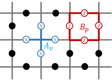
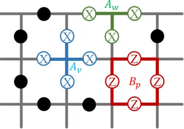
The toric code introduced by Kitaev [12] is a model of a system consisting of spins arranged in a two-dimensional lattice with continuous boundaries forming a torus (hence the name ‘toric’.) The spins are located at the edges of the lattice and are governed by local four-spin interactions involving X and Z Pauli matrices as shown in Figure 2.1. The interaction linking spins around vertices is called the vertex operator Av, and the one linking spins on plaquettes is the plaquette

operator Bp. The operators are defined as follows

Av = Y i∈v σ_ix, (2.1) Bp = Y j∈p σz_j, (2.2)

where v is the set of spins around the vertex v, and p being the set of spins around the plaquette p. The Hamiltonian is the sum of these interactions for all vertices

Z Z Z Z X X X X

𝐵

_𝑝

𝐴

_𝑣

Figure 2.1: The red square represents the Bp interaction linking the four spins

on the edges of plaquette p through σz_{. While the blue link represents the A} v

interaction linking the four spins on the vertex v through σx.

and plaquettes [15] H = −X v Av− X p Bp. (2.3)

For a lattice of size Lx × Ly, and the number of independent spins will be

2LxLy and the Hilbert space, denoted by H, will have a dimensionality of 22LxLy.

The general state of the toric code can be specified by specifying the state of each constituting spin in the basis chosen to be the eigenvectors of σz

|0i = 1 0 ! , |1i = 0 1 ! . (2.4)

For example, the state in which all spins are in the spin-up state |0i is denoted as

| ↑ · · · ↑i = |0i ⊗ · · · ⊗ |0i. (2.5) Similarly, all operators acting in the toric code Hilbert space are generated from

the basic definitions of the single-spin subspace operators with 1 = 1 0 0 1 ! , σx = 0 1 1 0 ! , σy = 0 −i i 0 ! , σz = 1 0 0 −1 ! . (2.6) An X Pauli matrix acting on the ith spin is defined as the Kronecker product of identities in the subspaces of all the other spins and σx _{in the subspace of the ith}

spin σx_i = 2LxLyterms z }| { 1 ⊗ · · · ⊗ 1 ⊗ · · · σx |{z} i-th term · · · ⊗ 1 . (2.7)

A vertex and plaquette operator can have either no shared spins, or two shared spins. This implies that, according to the anti-commutation relation {σα, σβ} = 2δαβ, any two vertex and plaquette operators will commute

[Av, Bp] = 0 ∀v, p. (2.8)

The Hamiltonian of the system is made up of mutually commuting operators that can be simultaneously diagonalized. The ground state is therefore the si-multaneous eigenstate of all Av and Bp with eigenvalue +1. A state that satisfies

this condition is [19] |ξ0i = Y v 1 √ 2(1v+ Av)| ↑ · · · ↑i. (2.9) Note that this state is the superposition of all possible products of Av operators

with equal weights. The ground state has an energy that depends on the number of vertices (Nv) and plaquettes (Np) which can also be expressed in terms of the

size of the system (Lx× Ly)

H|ξ0i = − X v Av− X p Bp ! |ξ0i = (−Nv− Np) |ξ0i (2.10) = −2LxLy|ξ0i (2.11) = E0|ξ0i. (2.12)

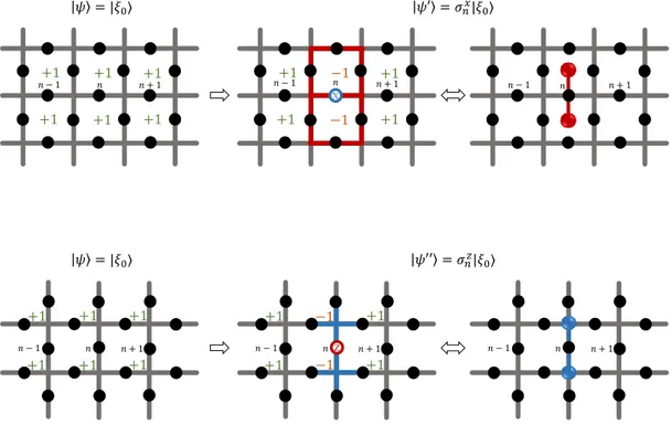
𝜓 = |𝜉₀⟩ 𝜓′ = 𝜎_𝑛𝑥_|𝜉 0⟩ +1 +1 +1 +1 +1 +1 𝑛 − 1 𝑛 𝑛 + 1 +1 +1 −1 −1 +1 +1 𝑛 𝑛 − 1 𝑛 + 1 X 𝑛 − 1 𝑛 𝑛 + 1 𝜓 = |𝜉0⟩ 𝜓′′ = 𝜎𝑛𝑧|𝜉0⟩ +1 +1 +1 +1 +1 +1 𝑛 − 1 𝑛 𝑛 + 1 +1 +1 +1 +1 𝑛 − 1 𝑛 𝑛 + 1 −1 −1 Z 𝑛 − 1 𝑛 𝑛 + 1

Figure 2.2: Starting from a ground state where all plaquettes (upper image) or vertices (lower image) measure an eigenvalue of +1 (leftmost image), then if σx or σz _{is applied to the n-th spin, the two plaquettes or vertices that share this}

spin will read an eigenvalue of −1. The eigenvalues of −1 are local and can be treated as “quasiparticles” (rightmost image.)

2.1.2

Excitations as quasiparticles

Starting from Eq. (2.9), it is possible to generate an excited state by applying either σx _{or σ}z _{to one of the spins. Take for example the following state}

|φi = σx

n|ξ0i, (2.13)

applying a plaquette operator Bp0 to |φi will be non-trivial only when n ∈ p0 so

that

Bp0|φi = B_p0σ_nx|ξ₀i = −σ_nxB_p0|ξ₀i = −σx_n|ξ₀i = −|φi, (2.14)

+1 +1 −1 −1 +1 +1 𝑗 𝑖 𝑘 X 𝑖 𝑗 𝑘 𝜙 = 𝜎_𝑖𝑥|𝜉0⟩ 𝜎𝑗 𝑥_|𝜙⟩ +1 +1 −1 −1 +1 +1 𝑗 𝑖 𝑘 X X 𝜎_𝑘𝑥_𝜎 𝑗𝑥|𝜙⟩ 𝑖 𝑗 𝑘 𝑖 𝑗 𝑘 +1 +1 −1 −1 +1 +1 𝑗 𝑖 𝑘 X X X

Figure 2.3: The transportation of a σx _{quasiparticle can be effectively done by}

applying a sequence of σx _{operators to spins connected to that spin through}

plaquettes. This new state constitutes a different, although degenerate, excited state.

σx. For any excitation σ_nx, there exists two plaquettes which overlap with the nth spin. The energy of the state |φi is then found to be

H|φi = −X v Av− X p Bp ! |φi = (−Nv − (Np − 2) + 2) |φi = (E0+ 4) |φi. (2.15)

The same argument applies for σz _{excitations which are detectable by A} v as

shown in Figure 2.2. Due to the locality of the excitations of this model it is useful to think of them as “quasiparticles.” An excitation at the nth edge creates two quasiparticles at the ends of that edge. Particles that are detectable (i.e. have eigenvalue −1) by Bp are called type ‘e’ and those detectable by Av are

called type ‘m.’ It follows that a state in which there are no quasiparticles (the ground state) is referred to as a ‘vacuum’ state.

If σx is applied at the ith edge and another excitation is applied at the jth edge which is connected to the ith edge through a plaquette, Bp with {i, j} ∈ p,

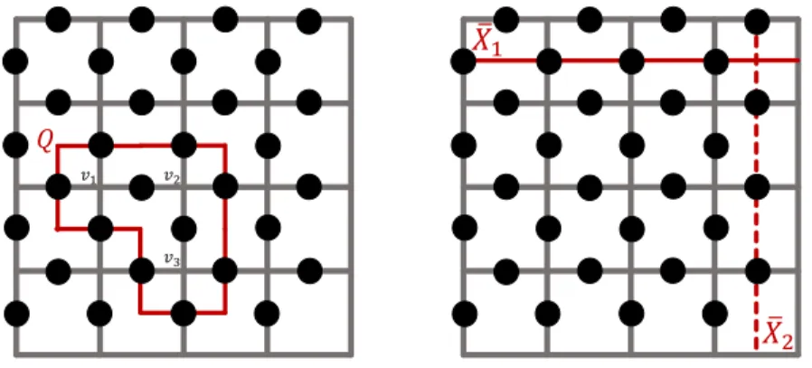
𝑣1 𝑣2 𝑣3 𝑄 ത 𝑋₂ ത 𝑋₁

Figure 2.4: The left image shows a trivially closed loop which is not detectable by any Bp operator and yet is deformable and removable by applying the vertex

operators Av1Av2Av3. The right image shows loops that close non-trivially in

the sense that while still being undetectable, they cannot be removed by any application of Av.

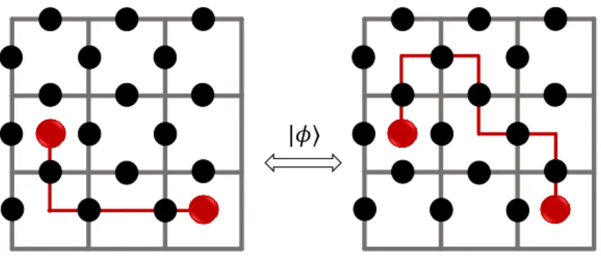
same type results in their annihilation. The quasiparticle was effectively trans-ported from one plaquette to a neighboring one (Figure 2.3.) Arbitrary transport operators consist of products of one or more than one connected excitations

ˆ

Ox_L=Y

j∈L

σx_j, (2.16)

where L is the path made up of spins that are connected through plaquettes. The same idea can be applied to the transportation of σz _{quasiparticles.}

If the path taken by these excitations winds up at the initial point, it forms a closed loop. Consider an arbitrary closed loop Q of σx excitations acting on the ground state in Eq. (2.9) as in the image on the left-hand side of Figure 2.4. This state is not detectable by Bp, ∀p. At the same time, the loop is deformable by

acting on it with vertex operators Av and if chosen properly, can be completely

removed. Such loops are called “contractible loops”.

Another way to look at it is that, since the ground state consists of the super-position all possible combinations of Av operators (or all possible loops formed

by them) according to Eq. (2.9), applying a contractible loop to the ground state will only cause a reshuffling of these underlying Av loops (i.e. turning one into

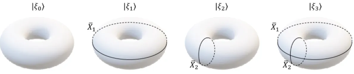
|𝜉0⟩ |𝜉1⟩ |𝜉2⟩ |𝜉3⟩ ത 𝑋1 ത 𝑋2 𝑋ത2 ത 𝑋1

Figure 2.5: Ground state subspace of the toric code

contractible loop,

ˆ

Q|ξ0i = |ξ0i. (2.17)

Similarly, an excited state in which two quasiparticles are fixed at the vertices (or equivalently, plaquette) v and v0 is made up of the superposition of all possible paths connecting these two end points. Application of any Av or Bp does not

result in the displacement of quasiparticles and only deforms the paths connecting them. Therefore, an excited state is distinct from another degenerate excited state if its quasiparticles are located at different points in the lattice. This is depicted in Figure 2.6.

2.1.3

The ground state subspace

Consider a loop ¯X1 that runs horizontally around the torus (Figure 2.4,

right-hand side image) It is not possible to remove ¯X1 using any combination of Av.

Such loops are called “non-contractible” loops. However, since the loop is closed, it does not entail any energetic penalty. We conclude that the resultant state is a distinct ground state. A loop running vertically ( ¯X2) constitutes another

degenerate ground state. Also, the combination of both horizontal and vertical loops is the fourth ground state. The ground state subspace is 4-dimensional. The degenerate ground state subspace of the toric code is shown in Figure 2.5.

|ξ1i = ¯X1|ξ0i, |ξ2i = ¯X2|ξ0i, |ξ3i = ¯X1X¯2|ξ0i. (2.18)

Such topologically non-trivial operators also exist for σz _{excitations and they}

do not produce a distinct state. This is because the operator ¯Z consists of σz

which, when acting on a single spin, only generates a phase and can not cause a spin flip. Therefore, ¯Z can not map the ground state to a different ground state.

The ground state subspace is used as the code space of the quantum device, i.e., the space in which logical information is encoded. Since the subspace is 4 dimensional, it is used to encode 2 qubits. Formally, the code subspace L is defined as follows:

L = {|ξi ∈ H : Av|ξi = |ξi, Bp|ξi = |ξi, ∀v, p} . (2.19)

In this code space, the logical operators, which can cause transitions between ground states, are the topologically non-trivial loop operators: { ¯X1, ¯X2}. The

application of a logical gate involves creating a pair of quasiparticles and walking one of them around a topologically non-trivial direction back to the other pair and annihilating them.

2.1.4

Errors and remedies

The presence of quasiparticles violates the condition Av|ξi = |ξi, Bp|ξi = |ξi

and takes the system out of the codespace and is therefore considered to be an “error.” Decoherence occurs as a result of the interaction between the system and the environment that causes these errors and eventually results in loss of the information stored in the quantum state.

Detecting errors is simply done by measuring the eigenvalues of all Av and Bp

operators. This set of eigenvalues s = {av, bp} is known as the error syndrome.

Due to the locality of these operators, the error syndrome provides information about the locations of the present quasiparticles. That being said, the error syndrome alone does not tell us all we need to know in order to remove the error. While we are able to tell the location of the quasiparticles, we do not know the details of the path connecting them. (Figure 2.4)

|𝜙⟩

Figure 2.6: Excited states are uniquely determined by the positions of the quasi-particles and are independent of the underlying path connecting them. Unless we track the time evolution of each quasiparticle, it is not possible to determine the path connecting them solely relying on the error syndrome.

one has to do is to annihilate the quasiparticles by closing the open loop in a topologically trivial manner such that the logical state is preserved. The invari-ance of the state under topologically trivial error loops is what makes the toric code passively error-correcting. If this annihilation of quasiparticles is done by closing the loop in a topologically non-trivial way, a logical error occurs where a transition to another ground state takes place and the stored information is altered, which is an undesired outcome. To avoid this, a correction process is im-plemented through a decoding algorithm. A decoder takes as an input the error syndrome and calculates the most probable error string and applies a correcting operator to remove the error while protecting the logical state [20]. That being said, a decoder has limitations.

To elaborate more on this point, consider the situation where the bit flip and phase errors happen with probability that is small enough such that the errors are dispersed in the lattice and the quasiparticle pairs have not walked far from each other [17]. Correcting for them in a topologically trivial way using the decoder becomes manageable. On the other hand, if that probability is large, predicting which quasiparticle pairs belong to each other and correcting for the error such that information is preserved becomes challenging. In this sense, the toric code is a fault-tolerant code in which errors can be reliably detected and removed if

the probability or rate of their occurrence is low enough.

To conclude, the error-correction properties of the toric code can be classified as: (1) passive, or (2) active. The passive error correction is the invariance of any ground state (or, in general, any energy eigenstate) under topologically trivial loops of excitations, while the active error correction is the use of a decoder to actively remove the errors in the system.

2.1.5

Modelling environment effects

In modelling the finite temperature dynamics of the toric code we need to in-troduce an auxiliary system known as the heat bath with which the toric code interacts. To proceed, a few assumptions need to be made. First, we assume that this heat bath is “Markovian” such that the heat bath is not affected by its inter-actions with the system. Second, we assume that the coupling between the heat bath and the system is weak. Finally, it is assumed that the heat bath-system interactions are local where each spin on the lattice is coupled independently to the heat bath.

We are interested in the evolution of the toric code (TC) in contact with a heat bath (B) under a Hamiltonian describing the combined closed system TC + B

H(t) = HTC⊗ 1B+ 1TC⊗ HB+ HI(t), (2.20)

where HI(t) is the system-bath interaction Hamiltonian. The information related

to the TC system can be extracted from its density matrix ρ =P

ipi|ψiihψi| where

pi ∈ [0, 1] is the statistical weight (or probability) of the corresponding state |ψii.

The time evolution of the density matrix of the open TC system is governed by the Lindblad master equation[21]

˙ ρ = −i

~[H, ρ] + Lρ, (2.21) where H is the TC Hamiltonian and L is the Liouvillian superoperator. The term

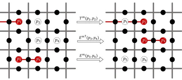
𝑝1 𝑝2 𝑝₃ 𝑝4 𝑝5 𝑝6 𝑝2 𝑝₃ 𝑝4 𝑝5 𝑝6 𝑝1 𝑇𝑚_(𝑝 1, 𝑝2) 𝐸𝑚†_(𝑝 3, 𝑝4) 𝐸𝑚_(𝑝 5, 𝑝6)

Figure 2.7: The possible events due to the environmental interactions are either translation Tm_{(p, p}0_{), creation E}m†_{(p, p}0_{), or annihilation E}m_{(p, p}0_).

are more interested in the dissipative dynamics described by the Liouvillian term

Lρ ≡X

i

LiρL†i − L †

iLiρ − ρL†iLi, (2.22)

where {Li} is the set of Lindblad or jump operators generated by the

system-environment interactions. In our case, the Lindblad operators will involve only single spin operations assuming local interactions between the system and the heat reservoir. These operators are then either single-spin translation T , anni-hilation E, or creation E† operators applied at rates γ0, γ− and γ+ respectively

(Figure 2.7.) For type ‘m’ quasiparticles, they are defined as

Tm(p, p0) = 1 4σ x pp0(1 − B_p) (1 + B_p0) , Em(p, p0) = 1 4σ x pp0(1 − B_p) (1 − B_p0) , Em†(p, p0) = 1 4σ x pp0(1 + B_p) (1 + B_p0) . (2.23)

The corresponding operators for type ’e’ quasiparticles are identical with the replacements Bp → Av and σx → σz. If the system is initialized in an energy

eigenstate, then the action of these jump operators keeps the state of the system within the set of its energy eigenstates. As a result, the TC density matrix stays

diagonal in the energy basis throughout the time evolution. Based on this, and combining Eq. (2.21) and Eq. (2.25) while discarding the coherent term −i

~[H, ρ]

we arrive at a simplified equation governing the diagonal matrix elements of the density matrix ˙ Pn= X m6=n (γm→nPm− γn→mPn). (2.24)

We can go a step further by explicitly considering all three possibilities of state m where it can be a state n0 that is degenerate with n, or a state n+ which has

a higher energy eigenvalue than n or a state n− which is lower than n. In doing

so, we arrive at ˙ Pn = γ0 X n0 (Pn0 − Pn) + X n+ (γ−Pn+ − γ+Pn) + X n− (γ+Pn−− γ−Pn), (2.25)

For a heat bath characterized by an Ohmic power spectrum [22], the rates at which each jump operator occurs depend on the temperature (or β = 1/T ) of the heat bath and the energy difference (or energy barrier) ∆ε ≡ (εf − εi) between

the initial state and the final state connected by that operator

γ(∆ε) = ∆ε

eβ∆ε_{− 1}. (2.26)

It can be verified that the rates according to this equation satisfy the detailed balance that fixes the ratio γ+/γ−

γ+

γ−

= e−β∆ε, (2.27)

This guarantees that the TC system coupled to a heat bath will evolve to its equilibrium state described by the density matrix ρ(β) = _Z1 P

ie −βEi_|n

iihni|.

2.1.6

Low temperature dynamics

In this subsection, we argue that the dominant process that can cause a logical error at low T is that of a random walker of excitations [23, 18]. For a logical error to occur, a chain of excitations winding around the torus need to be applied

by the environment interactions ¯ X =Y

i∈C

σ_ix. (2.28)

Note that this operator is not unique; the excitations σx

i can be applied in any

order, or through another path C0 different from C by some combination of vertex operators. However, these possibilities are not equally likely with thermalization. An ordering of excitations in Eq. (2.28) which results in a lower energy barrier is more likely according to Eq. (2.26). Specifically, one can start with a single excitation (first excited state) and wind up around the torus through translation of these particles without extra energetic cost. Such a process minimizes the energy barrier required for a logical error and is thus the most likely process that occurs in the low T regime.

Motivated by this conclusion, we use the dynamics of a random walker on the TC system to study the scaling of its resilience to logical errors in the low T regime.

2.2

The cylindrical code

Here we propose a modification to the toric code in which the continuity is re-moved from the vertical direction of the surface and is kept horizontally, thus forming a cylindrical geometry. We want to investigate such a system and com-pare it to the toric code to see whether it is advantageous in some ways.

As we had previously, the spins are located at the edges of a lattice and are governed by plaquette and vertex interactions in the inner region. For a choice of lattice where all plaquette operators are chosen to be a 4-spin interaction, it is evident that there is a need to define modified three-spin vertex operator at the upper and lower boundaries

Aw =

Y

i∈w

σx_i, (2.29)

X

X

X

X

Z

Z

Z

Z

X

X

X

𝐴

𝐵

𝐴

Figure 2.8: The boundary necessitates the addition of a 3-spin interaction Aw in

addition to the original operators Av and Bp.

have that

[Aw, Av] = [Aw, Bp] = 0 ∀ w, v, p , (2.30)

since the operator Aw trivially commutes with all Av and can share either no spins

or two spins with Bp, therefore commutes with it. The Hamiltonian is given by

the sum of all of these interactions that are mutually commuting,

H = −X v Av − X w Aw− X p Bp. (2.31)

The vacuum state is the state for which the eigenvalues of all Av, Aw and Bp is

+1, mathematically given by |ξ0i = Y j∈v,w 1 √ 2(1j+ Aj) | ↑ · · · ↑i. (2.32) For a system of size Lx × Ly, we will have a total of 2LxLy + Ly spins and a

Hilbert space of dimension 22LxLy+Ly_{. The ground state energy can be written in}

terms on the Lx and Ly or the number of vertices and plaquettes in the system,

H|ξ0i = −(Nv + Nw + Np)|ξ0i (2.33)

As in the toric code, excited states can be generated by applying either σx_{, σ}z _or

both to a spin in the lattice since the same commutation relations hold. One of the main differences between the toric code and the cylindrical code lies in the energy spectrum. In the toric code we had that any excitation σx _{or σ}z _resulted

in the creation of two quasiparticles, that is, the eigenvalues of the two operators, vertex or plaquette, sharing the same spin become −1. This increases the energy by 4 units of energy. While this still holds in the cylindrical code for the inner spins, applying an excitation of σx _{to a boundary spin results in the creation of}

a single quasiparticle since that spin lies on the edge of a single plaquette. It can be shown that such a process increases the energy of the system by 2 units of energy.

Single quasiparticles created at the boundaries can only be annihilated there, since anywhere else two quasiparticles are created at a time. Also, these single particles can be transported on the lattice by applying a string or a path of excitations on the lattice, like we had previously in the toric code.

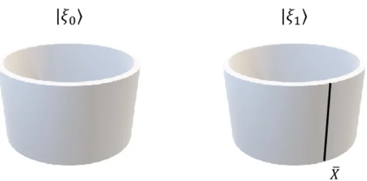
Now we address the degeneracy of the ground state. In this cylindrical ge-ometry the ground state subspace is two-dimensional where one of them is the vacuum state given by Eq. (2.32). While it is tempting to think that the other ground state will be the horizontal winding of quasiparticles, that is not the case. A horizontal winding (i.e. a closed path of σx excitations running along the cylinder horizonally) is indeed contractable in this cylindrical system by the modified vertex operators at the boundaries. Instead, a transition to the second ground state can be achieved by having a path of excitations ¯X run vertically from one open end of the cylinder to the other end. It can be verified that such a path is not contractable by any combination of vertex or plaquette operator and therefore results in a unique vacuum state

|ξ1i = ¯X|ξ0i. (2.36)

The logical operator ¯X is shown in Figure 2.9. This ground state subspace is used to store logical information and since it is two-dimensional, it can store 1 qubit. The codespace is defined as

|𝜉0⟩ |𝜉1⟩

ത 𝑋

Figure 2.9: The ground state subspace of the cylindrical code.

The passive error correction now is realized by the vacuum state’s invariance of all closed excitation loops including the horizontal windings and loops starting and ending at the same boundary. One of the main advantages of lowering the number of qubits encoded in the system is the possibility of having more effective active error correction. The main task of the decoder will be to connect stray quasiparticles in such a way that annihilates the ones that have originated in the boundaries back and the pairs that have originated within the surface together.

To simulate the interaction of the cylindrical system with the environment we look at the dynamics of it when in contact with a heat bath at temperature T . The same description outlined previously for the toric code holds except for the addition of events of single-quasiparticle creations and annihilation at the boundaries Em(w) = 1 2σ x w(1 − Bw) (2.38) Em†(w) = 1 2σ x w(1 + Bw) (2.39)

where w refers to the spin located at either, the upper or lower open boundaries of the cylindrical surface. Note that there is no single-quasiparticle e-type jump operators because σz _{quasiparticles are created in pairs everywhere on the lattice.}

At temperatures low enough we will have a higher probability of the creation of single quasiparticles at the boundaries compared to pairs within the surface

can propagate through the surface with no energy cost. Therefore, the dynamics governing the cylindrical code at low temperatures are those of a random walker starting from one boundary. A logical error is realized when the walker reaches the other side, and the original vacuum state is preserved if it returns to the same side.

2.3

Numerical methods

The aim of this section is to briefly describe the numerical methods used to derive the results in Chapter 3.

2.3.1

Random walker in 2D

Monte Carlo methods are best suited to simulate random processes such as the dynamics of a random walker and the probability that a walker results in a logical error. In the toric code, the walker consists of a pair of quasiparticles while in the cylindrical code we look at the dynamics of a single quasiparticle. Either way, we assume that the temperature is low enough so that no additional quasiparticles are created throughout the evolution which amounts to setting γ+= 0.

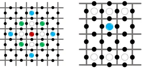
In the toric code, we keep one quasiparticle fixed and let the other move around the surface randomly as this is equivalent to having them both walk randomly since the relative motion is still random. The moving quasiparticle is initialized in a position that is one lattice spacing away from the fixed quasiparticle as shown in Figure 2.10. The moving quasiparticle is then left to walk randomly until it arrives at a position adjacent to the fixed quasiparticle where the trajectory is terminated since in practice the annihilation probability will be high at low temperatures. This is equivalent to working in the limit γ−→ ∞. Depending on the path taken,

this can result in a transition to another vacuum state if the number of windings along one or both directions is odd. Throughout the evolution, information about the windings is recorded to be able to identify walkers that resulted in a logical

Figure 2.10: The starting positions (blue and green) and annihilation positions (dashed) in the toric code (left image) and the cylindrical code (right image). In the toric code, the particle is started at either the blue or the green locations with the green locations being sampled twice as often as the blue locations due to their relative probability of occurrence. In the cylindrical code, the starting position is an arbitrary location along x (since they are all equally probable) and 1 lattice spacing below the upper boundary.

error.

In the cylindrical code, we initialize the system with a single quasiparticle that moves randomly around the lattice. Specifically, the starting position is 1 lattice spacing below the upper boundary (Figure 2.10) and the trajectory is terminated when the quasiparticle reaches an annihilation position at either the upper or lower boundaries. A logical error is registered if the particle reaches the lower boundary.

In both cases, the total number of steps n taken to for every trajectory is tracked. This process is repeated for many independent trajectory simulations to find the probability that a random walker ends up in a logical error

Probability of logical error (n) ≈ Number of runs ending up in a logical error (n) Total number of runs .

(2.40) It is evident that the larger the number of runs through which the system is

simulated the better this approximation becomes.

2.3.2

Continuous time Monte Carlo simulation of the

thermal evolution

The master equation governing the thermal evolution of the system given by Equation 2.25 can be simulated using a continuous time Monte Carlo method. To start, we note that the jump operators given by Equation 2.23 keep the sys-tem within the Hamiltonian eigenstate subspace. A general excited state can be uniquely specified by specifying the eigenvalues of all of the operators Av and Bp

(and Aw in the case of the cylindrical code.)

A trajectory of the system is evolved in time starting from an initial condition typically chosen as a ground state for a duration up to tmax. At each step of

the evolution an event V and a waiting time δt are chosen such that |ψ(t + δt)i = V |ψ(t)i. In the context of a surface code, these events constitute creation, annihilation and translation (Eq. (2.23)) of quasiparticles each of which has a rate of occurrence dependent on their corresponding energy barrier given by Eq. (2.26). The event is chosen based on the probability that it occurs which is calculated by

Probability(V ) = γ(V )

R (2.41)

where R is the sum of the rates of the processes that take the system out of the current state to another one, R =P

V ∈T ,E,E†γ(V ), evaluated with respect to

|ψ(t)i at each iteration. The waiting time δt is determined by

δt = −1

Rln r (2.42)

where r is a uniformly chosen number between 0 and 1. The event V is applied and the time evolved by δt and this process is repeated until t > tmax. Quantities

of interest are found by running many independent trajectories starting from the same initial condition and finding their average.

Chapter 3

Results and Discussion

3.1

Random walker

In order to gain insight into the low temperature dynamics of the toric code and how it compares to the cylindrical code, a discrete Monte Carlo simulation of a random walker on the surface is evolved for different system sizes. In the cylindrical system, the lattice is chosen to be continuous along the x direction, and open along y.

Typically, the toric code is studied in the context of a square lattice [18, 23] because of its continuity along both the x and the y directions. However, in this work we are interested in looking at how the dynamics change when an asymmetry between the two sizes is introduced. Therefore, we look at two cases: in one case, the system is kept as a square lattice in which the horizontal and vertical sizes X and Y are equal (i.e. X = Y ≡ L.) In the second case, we keep X constant and vary Y .

(a) X = Y = 4 100 ₁₀1 ₁₀2 10−8 10−6 10−4 10−2 n Ptransition (b) X = Y = 8 101 102 103 10−8 10−6 10−4 10−2 n Ptransition (c) X = Y = 12 101 ₁₀2 ₁₀3 10−8 10−6 10−4 n Ptransition (d) X = Y = 16 101 102 103 10−8 10−6 10−4 n Ptransition Toric Cylindrical

Figure 3.1: The average number of steps that end up in a logical error as a function of system size for the case X = Y .

3.1.1

Transition probability vs. the number of steps

Figures 3.1a, 3.1b, 3.1c and 3.1d depict the probability of a logical error Ptransition

as a function of the number of steps taken by the walker for the toric and cylin-drical codes with X = Y = L. It can be seen that while the two curves behave similarly in the small n regime, they deviate quite notably for larger n where the cylindrical code shows a drop in the transition probability. Also, the step number at which Ptransitionis maximum becomes evidently lower (shifts to the left) for the

(a) X = 4, Y = 8 100 ₁₀1 ₁₀2 10−8 10−6 10−4 10−2 n Ptransition (b) X = 4, Y = 12 100 ₁₀1 ₁₀2 ₁₀3 10−8 10−6 10−4 10−2 n Ptransition (c) X = 4, Y = 16 100 ₁₀1 ₁₀2 ₁₀3 10−8 10−6 10−4 10−2 n Ptransition Toric Cylindrical

Figure 3.2: The average number of steps that end up in a logical error as a function of system size with X = 4 and Y = {8, 12, 16}.

that, when working in a square lattice, the cylindrical code becomes advantageous for larger system sizes.

Figures 3.2a, 3.2b and 3.2c show the effect of varying the vertical size of the system Y while keeping the horizontal size X fixed. As for the toric code, this poses a severe disadvantage since a walker can quickly result in an odd winding along the shorter distance, namely X, with a high probability which explains the behaviour of the toric code curve at small n (Figure 3.2.) The cylindrical code avoids this altogether since it is concerned solely with the vertical size Y for a logical error to occur. For this reason we see that the cylindrical code walker dynamics for both fixed X and varied X are identical as long as Y is the same.

(a) X = Y = L 0.3 0.4 0.5 0.6 0.7 0.8 0 0.2 0.4 [ln L]−1 Ptransition (b) X = 4, Y varied. 0.3 0.4 0.5 0.6 0.7 0.8 0 0.2 0.4 [ln Y ]−1 Ptransition Toric Cylindrical

Figure 3.3: The total transition probability as a function of system size.

3.1.2

Transition probability vs. system size

The total transition probability is found by summing over n and is plotted in Figure 3.3 as function of system size. In both figures we see that the cylindrical code provides better resilience against logical errors by having a lower transition probability for all system sizes. The result of varying Y is shown in Figure 3.3b where the gap in transition probability between the cylindrical and toric codes has significantly increased as compared to the square lattice case in Figure 3.3a.

To quantify this behaviour we fit the transition probability to a function of the form

Ptransition(L) = a +

b

ln L (3.1)

where a and b are constants to be determined. This form derives from the phe-nomenology of a random walker in 2D in which the probability that a walker does not return to its starting point after m steps scales as 1/ ln m [24]. Applying this to our model, we need that, on average, the walker does not return to the origin before surpassing the relevant system size squared for a logical error to occur. That is, we expect a scaling of the form [2 ln L]−1. From the fittings we find that

(a) X = Y = L 100.6 ₁₀0.8 ₁₀1 ₁₀1.2 100 101 102 L ¯n (b) X = 4, Y varied. 100.6 100.8 101 101.2 100.5 101 Y ¯n Toric Cylindrical

Figure 3.4: The average number of steps that end up in a logical error as a function of system size.

the data closely matches the fits given by

Ptor(L) = −0.08 + 1.32 ∗ [2 ln L]−1 (3.2)

Ptor(Y ) = +0.25 + 0.38 ∗ [2 ln Y ]−1 (3.3)

Pcyl(L) = −0.21 + 1.50 ∗ [2 ln L]−1 (3.4)

3.1.3

Average step number vs. system size

We look at the average number of steps required for a logical error to occur for different system sizes. The average number of steps is found by calculating ¯

n =P

nnP (n). The expected behaviour is a monotonic increase of ¯n with system

size. Indeed, as shown in figures 3.4a and 3.4b, the average step number very closely fits a power law of the form

¯

ntransition(L) = aLb (3.5)

• ator = 0.48, btor = 1.10 for X 6= Y , and

• acyl = 0.38, bcyl= 1.18.

Comparing ¯n for the two systems gives us an insight into the relative average time it takes for a logical error to occur. When X = Y it is evident that it takes less steps on average for a logical error to occur in the cylindrical code than it takes in the toric code. This can be attributed to the fact that the number of annihilation positions available in the cylindrical code increases with the horizontal size X, while independent in the toric code. It follows that the walker in the cylindrical code is more likely to annihilate with a smaller number of steps. Figure 3.4b shows that this gap shrinks significantly when X is fixed and Y is varied since the effect of the increase in X is now eliminated.

Chapter 4

Conclusion

In light of the above discussion we can say that the cylindrical system is generally more resilient to logical errors in the zero temperature limit. More so if an asymmetry in the horizontal and vertical system sizes is introduced where the system is longer in the direction of open boundaries. Doing that will also improve the average time it takes for a logical error to occur for the cylindrical code.

The geometry of a torus, as one would expect, can pose a challenge in experi-mental implementation. Therefore, it can be very useful to define modifications that provide easier experimental accessibility in terms of applying logical gates and reading logical information. We believe that the practical feasibility of the cylindrical geometry over a toric one is one of its main advantages.

That being said, it remains true that the codespace suffered as a result where the toric code can encode 2 qubits while the cylindrical code encodes 1 qubit. Despite this trade-off, the smaller code space and the fact that the creation and annihilation of single quasiparticle is restricted to the open boundaries makes the cylindrical code advantageous when active error-correction is taken into consid-eration.

method. Useful information about the temperature dependence of the coherence time can be extracted. Also, it would be interesting to implement a decoding algorithm and use that to estimate the accuracy threshold of the two systems and compare them.

Bibliography

[1] R. P. Feynman, “Simulating physics with computers,” Int. J. Theor. Phys, vol. 21, no. 6/7, 1982.

[2] S. Lloyd, “Universal quantum simulators,” Science, pp. 1073–1078, 1996. [3] P. W. Shor, “Polynomial-time algorithms for prime factorization and discrete

logarithms on a quantum computer,” SIAM review, vol. 41, no. 2, pp. 303– 332, 1999.

[4] C. H. Bennett and G. Brassard, “Quantum cryptography: Public key distri-bution and coin tossing,” arXiv preprint arXiv:2003.06557, 2020.

[5] J. Preskill, “Reliable quantum computers,” Proceedings of the Royal Soci-ety of London. Series A: Mathematical, Physical and Engineering Sciences, vol. 454, no. 1969, pp. 385–410, 1998.

[6] E. Knill, R. Laflamme, and W. H. Zurek, “Resilient quantum computation: error models and thresholds,” Proceedings of the Royal Society of London. Se-ries A: Mathematical, Physical and Engineering Sciences, vol. 454, no. 1969, pp. 365–384, 1998.

[7] P. W. Shor, “Scheme for reducing decoherence in quantum computer mem-ory,” Phys. Rev. A, vol. 52, pp. R2493–R2496, Oct 1995.

[8] D. A. Lidar and T. A. Brun, Quantum error correction. Cambridge university press, 2013.

[10] R. Barends, J. Kelly, A. Megrant, A. Veitia, D. Sank, E. Jeffrey, T. C. White, J. Mutus, A. G. Fowler, B. Campbell, et al., “Superconducting quantum circuits at the surface code threshold for fault tolerance,” Nature, vol. 508, no. 7497, pp. 500–503, 2014.

[11] A. D. C´orcoles, E. Magesan, S. J. Srinivasan, A. W. Cross, M. Steffen, J. M. Gambetta, and J. M. Chow, “Demonstration of a quantum error detection code using a square lattice of four superconducting qubits,” Nature commu-nications, vol. 6, no. 1, pp. 1–10, 2015.

[12] A. Y. Kitaev, “Fault-tolerant quantum computation by anyons,” Annals of Physics, vol. 303, no. 1, pp. 2–30, 2003.

[13] D. Bacon, “Operator quantum error-correcting subsystems for self-correcting quantum memories,” Physical Review A, vol. 73, no. 1, p. 012340, 2006. [14] C. Nayak, S. H. Simon, A. Stern, M. Freedman, and S. D. Sarma,

“Non-abelian anyons and topological quantum computation,” Reviews of Modern Physics, vol. 80, no. 3, p. 1083, 2008.

[15] J. K. Pachos, Introduction to topological quantum computation. Cambridge University Press, 2012.

[16] S. B. Bravyi and A. Y. Kitaev, “Quantum codes on a lattice with boundary,” arXiv preprint quant-ph/9811052, 1998.

[17] E. Dennis, A. Kitaev, A. Landahl, and J. Preskill, “Topological quantum memory,” Journal of Mathematical Physics, vol. 43, no. 9, pp. 4452–4505, 2002.

[18] C. D. Freeman, C. Herdman, D. J. Gorman, and K. Whaley, “Relaxation dynamics of the toric code in contact with a thermal reservoir: Finite-size scaling in a low-temperature regime,” Physical Review B, vol. 90, no. 13, p. 134302, 2014.

[19] M. Araujo de Resende, “A pedagogical overview on 2d and 3d toric codes and the origin of their topological orders,” Reviews in Mathematical Physics, vol. 32, no. 02, p. 2030002, 2020.

[20] J. Wootton, “A simple decoder for topological codes,” Entropy, vol. 17, no. 4, pp. 1946–1957, 2015.

[21] H.-P. Breuer, F. Petruccione, et al., The theory of open quantum systems. Oxford University Press on Demand, 2002.

[22] U. Weiss, Quantum dissipative systems, vol. 13. World scientific, 2012.

[23] B. J. Brown, D. Loss, J. K. Pachos, C. N. Self, and J. R. Wootton, “Quantum memories at finite temperature,” Reviews of Modern Physics, vol. 88, no. 4, p. 045005, 2016.

[24] F. Montalenti and R. Ferrando, “Probability of dimer reassociation in two dimensions,” Phys. Rev. E, vol. 61, pp. 3411–3416, Apr 2000.