Identifying probability distributions using neural networks

(1)

ІРЛ ЭВАВІІІТУ DiSTfälSUTäOW·'

US3?ü‘S MSUHAL î‘J£T»yjOf!ICS

« d

b

~~j İ.A W

m

4^'

.«Ч y . .

# ·! ■ Г

^ sUt/ ·<^ . V X

T h £ İ H S T İ T U T Î OP

'ВСОНОШСѢ

A - . i J !

O P ¿ l U l S K T У Н З Ѵ Р Е 2 І 7 ¥

( s ^ r

λ }

«1 ' '' .<41 r - j C “ r - u ^ ‘ » Ä ·-' M** Ы •N -^ « W .M U i ' ,--· ‘ j 1·=* T " ^ J U U ічМ Mm m.< U » Ш ) mJÉ 4 - ^ -i ‘ У і:· ^ tf· Vr '1 Д y ’ » *“ · w «i Ъ> w - w

· Я

" / у у

ÍS)

и

^

H G

¿ f

5 ”

V

4 5

· f Q

3 S

(2)

USING NEURAL NETWORKS

A TH ESIS

SU B M IT T E D TO

THE

D E PA lT l'M E N T OF E C O N O M IC S

A N D TH E IN ST IT U T E OF E C O N O M IC S A N D SO C IA L SC IE N C E S

OF B IL K E N T U N IV E R S IT Y

IN P A R T IA L FU L FIL L M E N T OF TH E R E Q U IR E M E N T S

FO R TH E D E G R E E OF'

M A ST E R OF A R T S

By

Anil Yılmaz

September 1995

hibrSLiW

...

VilM ay

...

€aicr/-c^zc:w:i·

c c/

■

(3)

Ц 5 И 5 .

5 • V 4 > o

< Ь Э 5

(4)

Asst. (Prof Faruk Selçuk (Supervisor)

I certify that I have read this thesis and that in my opinion it is fully adequate,

in scope and in quality, as a thesis for the degree o f Master o f Arts.

_

(c 't I

i i i

...¿-1

Assoc. Prof İhsan Sabuncuoğlu (Co-supervisor)

I certify that I have read this thesis and that in my opinion it is fully adequate,

in scope and in quality, as ^<^iqsis for A e degree o f Master o f Arts.

il-Assoc. P rof Pranesh Kumar

Approved for the Institute o f Economics and Social Sciences

/ y / y

Prof Ali L. Karaosmanoglu

Director o f Institute o f Economics and Social Sciences

(5)

A B ST R A C T

IDENTIFYING

PROBABILITY DISTRIBUTIONS

USING NEURAL NETWORKS

Anil Yılmaz

M.A. in Economics,

Supervisor; Faruk Selçuk

September 1995

Economics deal with real life phenomena by constructing representative models

o f the system being questioned. Input data provide the driving force for such models.

The requirement o f identifying the underlying distributions o f data sets is encountered

in econom ics on numerous occasions. Most o f the time, after the collection o f the raw

data, the underlying statistical distribution is sought by the aid o f nonparametric

statistical methods. At this step o f the problem, the feasibility o f using neural networks

for identification o f probability distributions is investigated. Also, for this purpose, a

comparison with the traditional goodness o f fit tests is carried out in this study.

Keywords: Neural Networks, Identifying Distributions, Goodness-of-fit.

(6)

İSTATİSTİKİ DAĞILIMLARIN

BELİRLENMESİ

Anıl Yılmaz

İktisat Yüksek Lisans

Tez Yöneticisi: Faruk Selçuk

Eylül 1995

Ekonomi bilimi gerçek hayattaki problemleri, bunları temsil eden modeller

kurarak inceler. Bu modellerin geçerliliğini modellere girdi oluşturan veriler sağlar.

Veri kümelerinin istatistiki dağılımlarının belirlenmesi gereksinimi ekonomide birçok

kez karşılaşılan bir durumdur. Genellikle ham verilerin toplanmasından sonra,

parametrik olmayan metodlarla istatistiki dağılım belirlenmeye çalışılmaktadır.

Problemin bu aşamasında yapay sinir ağlannın kullanımının mümkün olup olmadığı

araştınimıştır. Ayrıca, yine bu amaçla, uyum iyiliği testleri ile yapay sinir ağları

karşılaştırılmıştır.

Anahtar Kelimeler: Sinir Ağlan, Dağılım Belirleme, Uyum İyiliği.

(7)

1 INTRODUCTION

₁

2 ARTIFICIAL NEURAL NETWORKS

₃

2.1 Introduction

₃

2.2 History of Neural Networks

₅

2.3 Main Application Areas

₆

3 LITERATURE REVIEW

₇

4 SETTING

9 4.1 Distributions Selected

₉

4.2 Training Sets

₁₁

4.3 Probabilistic Neural Network (PNN)

₁₆

4.4 Counter Propagation Network

₁₉

4.5 Network Architectures

₂₁

4.6 Training the Networks

₂₂

5 RESULTS

24 6 CONCLUSION

31 APPENDIX A - Training Sets

33 APPENDIX B - Computer Programs

45 APPENDIX C

51 APPENDIX D - Recall Sets

53

(8)

2 Distributions Used

9 3 Assum ed Mininrum and Maximum Values o f Distributions

14 4 Percentage o f Distributions/Types Correctly Identified (PNN)

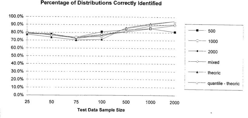
27 5 Percentage o f Distributions Correctly Identified (PNN)

28 6 Percentage o f Distributions/Types Correctly Identified (Counter)

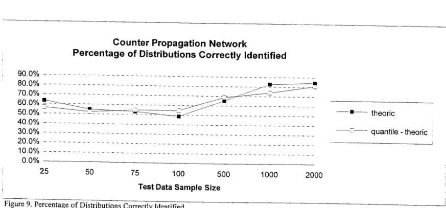
29 7 Percentage ofDistributions Correctly Identified (Counter)

30 A A l

Theoric Training Set (without quantiles)

34 AA2

Training Set for Sample Size 500 (without quantiles)

35 AA3 Training Set for Sample Size 1000 (without quantiles)

38 AA4 Training Set for Sample Size 2000 (without quantiles)

41 AA5

Theoric Training Set with Quantiles

44 ADI Recall Set with Quantiles for Sampe Size 25

54 AD2 Recall Set with Quantiles for Sampe Size 50

57 AD3

Recall Set with Quantiles for Sampe Size 75

60 AD4 Recall Set with Quantiles for Sampe Size 100

63 AD5

Recall Set with Quantiles for Sampe Size 500

66 .

AD6

Recall Set with Quantiles for Sampe Size 1000

69 AD7

Recall Set with Quantiles for Sampe Size 2000

72

(9)

List of Figures

1 A Typical Processing Element

3

2 A Simple Neural Network Arehitecture

4

3 Distributions Used

10

4 Structure o f a Typical Probabilistic Neural Network with 3 Features

and 2 Classes

18

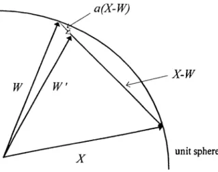
5 Adjustment o f W eights by the Kohonen Learning Rule

20

6 Percentage o f Distributions/Types Correctly Identified (PNN)

27

7 P e rc e n ta g e

o f Distributions Correctly Identified (PNN)

28

8 Percentage o f Distributions/Types Correctly Identified (Counter)

29

9 P e rc e n ta g e

o f Distributions Correctly Identified (Counter)

30

(10)

Econom ics deal with real life phenomena by constmcting representative models o f

the system being questioned. Input data provide the driving force for such models. The

requirement o f identifying the underlying distributions o f data sets is encountered in

econom ics on numerous occasions. Since modeling and simulation are frequently

em ployed techniques in econom ics, the problem o f hypothesizing the distribution o f a data

set is a major concern.

Many examples supporting the significance o f this issue can be illustrated. For

instance, suppose w e are faced with a game where the players are playing according to

som e mixed strategy by attributing probability distributions over a continuous choice set.

Having the past data on how the players respond, we seek for a solution o f the game by

conducting a Monte-Carlo simulation. Such an attempt would require the knowledge o f the

distributions that yield the players’ strategies.

As an example in the field o f macroeconomics, the necessity to find underlying

probability distributions may arise for incorporating external agents’ effects into a model.

In the case o f stochastic macroeconomics, in a setup with a continuum o f sates, probability

density function o f consumption becomes significant for determining the demand for

m oney which, according to Tobin (1958), is emerging partly as a result o f wealthholders’

desire to diversify their holdings.

Most o f the time, after the collection o f the raw data, the underlying statistical

distribution is sought by the aid o f nonparametric statistical methods. At this stage o f the

problem, the feasibility o f using neural networks for identification o f probability

distributions is investigated. A lso, for this purpose, a comparison with the traditional

goodness o f fit tests is carried out in this study.

Chapter 2 introduces the artificial neural networks and explains basic concepts.

Then a brief history o f neural networks together with main application areas is given. In

Chapter 3, the relevant literature on statistical and other related applications o f neural

networks is reviewed. Chapter 4 describes the main work done in this study. A more

detailed discussion o f the networks used, namely probabilistic and counter propagation

(11)

Chapter 1. Introduction

networks, is included in this chapter. Neural network architectures, probability

distributions, structure o f the data presented to the networks and the training process are

explained. The results and comparison o f the neural networks with the goodness-of-fit tests

are given in Chapter 5. Finally Chapter 6 contains concluding remarks and suggestions for

further research.

(12)

2.1 Introduction

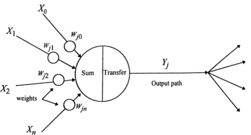
In an artificial neural network, the unit analogous to the biological neuron is

referred to as a “processing elem en f’. A processing element has many input paths and

combines, usually by a sim ple summation, the values o f these input paths. The result is an

internal activity level for the processing element. The combined input is then modified by a

transfer function. This transfer function can be a threshold function which only passes

information if the combined activity level reaches a certain level, or it can be a continuous

function o f the combined input. The output value o f the transfer function is generally

passed directly to the input path o f the next processing element.

The output path o f a processing element can be connected to input paths o f other

processing elements through connection weights which correspond to the synaptic strength

o f neural connections. Since each connection has a corresponding weight, the signals on

the input lines to a processing element are modified by these weights prior to being

Slimmed.

Thus, the summation function is a weighted summation. A typical processing

element is shown in Figure 1.

(13)

A neural network consists o f many processing elements joined together in the

above manner. Processing elements are usually organized into groups called layers. A

typical network consists o f a sequence o f layers with full or random connections between

successive layers. Generally, there are two layers o f special interest: an input layer where

the data is presented to the network, and an output layer which holds the response o f the

network to a given input. The layers between the input and output layers are called hidden

layers. A simple neural network architecture is shown in Figure 2.

Chapter 2. Artificial Neural Networks

4 There are tw o main phases o f operation o f a network: learning and recall phases. In

m ost networks these are distinct.

Learning is the process o f adapting or modifying the connection weights in

response to stimuli being presented at the input layer and optionally the output layer. A

stimulus presented at the output layer corresponds to a desired response to a given input.

This desired outcome m ust be provided to the network. Such type o f learning is called

“supervised learning”.

I f the desired output is different from the input, the trained network is referred to as

a hetero-associative network. If, for all training examples, the desired output vector is equal

to the input vector, the trained network is called auto-associative. I f no desired output is

shown the learning is called unsupervised learning.

A third kind o f learning is reinforcement learning where an external teacher

indicates only whether the response to an input is good or bad.

(14)

Me Culloch and Pitts (1943) represented the first formalized neural network model

consisting o f simple two state units in their paper called “A Logical Calculus o f Ideas

Imminent in Neural A ctivity.” which was an inspiration for studies forming the basis o f

artificial intelligence and expert systems.

Frank Rosenblatt, in 1957, published the first major research project in neural

computing: the development o f an element called a “perceptron” which was a pattern

classification system that could identify both abstract and geometric patterns. Perceptron

w as capable o f making limited generalizations and could properly categorize patterns

despite noise in the input.

In 1959, Bernard Widrow developed an adaptive element called “adaline”

(/fJuptive L/near Acuron), based on simple neuron-like elements. The Adaline and a two-

layer variant, the “madaline” (Multiple

Adaline)

were used for a variety o f applications

including speech recognition, character recognition, weather prediction and adaptive

control.

In the mid 1960s, Marvin Mirsky and Seymour Papert analyzed in depth the single

layer perceptrons and published the result in their book “Perceptrons” in 1969. They

proved that such networks were not capable o f solving the large class o f nonlinear

separable problems. They showed that extension o f hidden units would overcom e these

limitations, but stated that training such units was unsolvable. The conclusion o f this work

led to the decrease o f interest in the field o f neural networks and only a few researchers

continuing their work remained in the field.

It was in 1982, that John Hopfield represented a paper about a computing system

consisted o f interconnected processing elements that minimizes a given energy function

until the network stabilizes at a local or global minimum. Hopfield’s model illustrated

memory as information stored in the interconnections between neuron units. With the

introduction o f this paper, the field attracted substantial attention again.

(15)

Geoffrey Hinton and Terrence Sejnowski have developed the Boltzmann machine

in 1983, which used a stochastic update rule allowing the system to escape from local

minima. Two years later Rumelhart, Hinton and Williams derived a learning algorithm for

perceptron networks with hidden units based on Widrow-Hoff learning rule. This algorithm

called “back propagation" is one o f the most commonly used learning algorithms today.

Chapter 2. Artificial Neural Networks

5 2.3 Main Application Areas

Inspired by the biological systems, neural networks tend to be good at solving

problems in the areas o f statistics, modeling, forecasting, pattern recognition, pattern

classification, pattern completion, linear regression, polinomial regression, curve fitting

and signal processing.

Neural networks are employed in diverse fields such as chemical process control,

seismic exploration, vision-based industrial inspection, adaptive process control, machine

diagnostics, medical diagnostics, anti-body detection, classifying tissue samples, targeted

marketing, product marketing, financial modeling, forecasting, risk management, credit

rating, bankruptcy prediction, handwritten character recognition, speech recognition,

adaptive flight control, solar signal processing, coin grading, monitoring rocket valve

operations, race-track betting, etc.

One o f the new application areas for neural networks is to find near optimal

solutions for the combinatorial optimization problems.

(16)

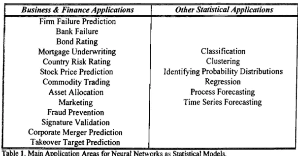
White (1989b) discusses the relationships between neural networks and traditional

statistical applications. As stated by Sharda (1994), in many papers, neural netw'orks have

been proposed as substitutes for statistical approaches to classification and prediction

problems. The conclusion derived from those papers suggest that neural networks'

advantages in statistical applications are their ability to classify where nonlinear separation

surfaces are present, robustness to probability distribution assumptions and ability to give

reliable results even with incomplete data. Neural networks are experimented in the major

areas o f statistics: regression analysis, time series prediction and classification. Thus neural

networks may be employed where regression, discriminant analysis, logistic regression or

forecasting approaches have been used. Marquez (1992) has provided a com plete

comparison o f neural networks and regression analysis. His results confirm that the neural

networks can do fairly w ell in comparison to regression analysis. The prediction capability

o f neural networks has been studied by a large number o f researchers. In early papers,

Lapeds and Färber (1987) and Sutton (1988) offered evidence that the neural m odels were

able to predict time series data fairly well. Many comparisons o f neural networks and tim e

series forecasting techniques, such as the Box-Jenkins approach have been reported. The

topics on which application papers describing neural networks as statistical m odels are

listed in Table 1.

Business & Finance Applications

Other Statistical Applications

Firm Failure Prediction

Bank Failure

Bond Rating

Mortgage Underwriting

Classification

Country Risk Rating

Clustering

Stock Price Prediction

Identifying Probability Distributions

Commodity Trading

Regression

Asset Allocation

Process Forecasting

Marketing

Time Series Forecasting

Fraud Prevention

Signature Validation

Corporate Merger Prediction

Takeover Target Prediction

(17)

Chapter 3. Literature Review

₈

The literature on the application o f neural networks to identifying probability

distributions is very limited.

Sabuncuoglu et al. (1992) investigated possible applications o f neural networks

during the input data analysis o f a simulation study. Specifically, counter propagation and

back propagation networks were used as the pattern classifier to distinguish data sets from

three basic distributions: exponential, uniform and normal. Histograms consisting o f 10

equal width intervals were used as input vectors in the training set. The performance o f the

networks was also compared to som e o f the standard goodness-of-fit tests for samples o f

different sizes and parameters. It was observ'ed that neural networks did not give exact

answers for data sets o f size 10. Goodness-of-fit tests were not powerful for small samples

either. They failed to reject any hypothesis when the sample size is small. The results for

samples o f size greater than 25 showed that using neural networks is a feasible method for

distribution identification. It is also noted that their study was limited in terms o f the

distributions investigated and much more effort might be necessary when other statistical

distributions are included in the study.

Akbay et al. (1992) proposed a method based on quantile information to assess the

applicability o f artificial neural networks to recognize certain patterns in raw data sets.

They compared the predictions o f a probabilistic and a feedforward (backpropagation)

neural network with the results from traditional statistical methods. Nine equal interval

normalized quantile values were used as the input and 25 different categories o f

distributions were presented to the networks as the training set. As stated in this research,

the probabilistic neural network (PN N ) learned (was able to correctly identify) all the 25

categories in the training set whereas the backpropagation network was able to learn 24 o f

the categories.

The trained networks were tested by 13 different data sets o f which the underlying

distributions were validated by using the goodness o f fit tests. It is concluded that the

preliminary results demonstrate that neural networks may be able to identify the fam ily o f

standard probability distributions. Nevertheless, there is the requirement that the selections

o f the neural netw’orks should be confirmed by the standard goodness-of-fit tests since

there were some cases in which the neural networks failed to identify the proper

distribution.

(18)

4.1 Distributions Selected

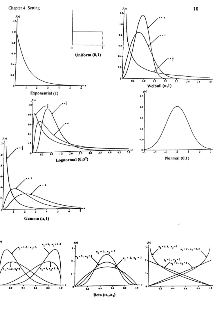
There are seven distinct distributions considered in this research: Uniform,

Exponential, Weibull, Gamma, Lognormal, Normal and Beta. Based on the different shape

parameters, there are also three types o f W eibull, Gamma and Lognormal distributions.

Similarly eleven different types o f Beta distribution are considered corresponding to

different shape parameters. Thus a total o f 23 categories are fonned for the networks to

classify among. These distributions are listed in Table 2 and graphed in Figure 3.

Distribution

number

/T yp e

Parameters

1 Uniform

m in=0, m ax=l

2 Exponential

location=0, shape=l

3 W eibull-1

location=0, sca le= l, shape=0.5

4 W eibull-2

location=0, sca le= l, shape=2

5 Weibull-3

location=0, sc a le = l, shape=3

6 Gam m a-1

location=0, sca le= l, shape=0.5

7 Gamma-2

location=0, sca le= l, shape=2

8 Gamma-3

location=0, sca le= l, shape=3

9 Lognorm al-1

location=0, scale=0, shape=0.5

10 Lognormal-2

location=0, scale=0, shape=l

11 Lognormal-3

location=0, scale=0, shape=1.5

12 Normal

mean=0, variance=l

13 B eta-1

m in=0, m a x = l, shapel=1.5, shape2=5

14 Beta-2

m in=0, m a x = l, shapel=1.5, shape2=3

15 Beta-3

m in=0, m a x = l, shape 1=5, shape2=1.5

16 Beta-4

m in=0, m a x = l, shapel=3, shape2=1.5

17 Beta-5

m in=0, m a x = l, shape 1=3, shape2=3

18 Beta-6

m in=0, m a x = l, shape 1=5, shape2=5

19 Beta-7

m in=0, m a x = l, shape 1=2, shape2=2

20 B eta-8

m in=0, m a x = l, shaj>el=0.8, shape2=2

21 Beta-9

m in=0, m a x = l, sh a p el= l, shape2=2

22 B eta-10

m in=0, m a x = l, shapel=2, shape2=0.8

23 B eta-11

m in=0, m a x = l, shapel=2, shape2=l

Table 2. Distributions Used.

(19)

/U)

Gamma (a,1)

(20)

In order to hypothesize appropriate families o f distributions o f a raw data set,

various heuristics

are used. Prior knowledge about the random variable, summary

statistics, histograms and line graphs, quantile summaries and box plots are used for this

purpose. Most commonly referred summary statistics include the minimum, maximum,

mean, median, variance, coefficient o f variation, skewness, etc.

In this study, based on our pilot experiments, skewness, quantile and cumulative

probability information are used to distinguish the distributions from each other. The

skewness

v

is a measure o f the symmetry o f the distribution. For symmetric distributions

lik e Normal or special types o f Beta, v=0. If v>0, the distribution is skewed to the right; i f

v<0, the distribution is skewed to the left. Thus the estimated skewness can be used to

ascertain the shape o f the underlying distribution. The quantile summary is also a synopsis

o f the sample that is useful in determining whether the underlying probability density

function is symmetric or skewed to the right or left. Inspired by the Q-Q and P-P plots,

quantile and cumulative probability values are used in the training set. Probability plots

lik e Q-Q and P-P plots, can be thought o f as a graphical comparison o f an estimate o f the

true distribution function o f the data with the distribution function o f the estimated

distribution. The quantile and the cumulative probability values are taken for points

concentrated on the left tail o f the density function. This is because the differences between

distribution functions o f different densities get smaller as we move along the x-axis.

Both empirical and théorie data are used as training sets. For the empirical case,

random variates o f sample size 500, 1000 and 2000 are generated by using SIMAN

simulation software package and UNIFIT II (Law & Associates-1994) statistical software

package. For each distribution/type, 5 data sets are generated; which makes a total o f 115

data sets for each sample size (5 data sets for each distribution/type

x

23 distiibutions/types).

Thus in each empirical training set there are 115 examples. Each example is

represented by a row containing the skewness, quantile values and cumulative probability

values. Also for each example (or row) in the training set, the desired output is given as a

sequence o f zeros and ones. This sequence contains 22 zeros and one “ 1” in the

(21)

Chapter 4. Setting

12 corresponding place for the correct distribution number in Table 2. A “ 1” in the first place

indicates that the example is from unifomi distribution, whereas normal distribution is

represented by a “ 1” in 12th place. An example row from a training set is given below.

Quantile Values (in percent)

Skewness

Q2.5

Q5

QI

Q12.5

Q2S

Q50

Q75

Q90

0.5373

0.143788

0.227522

0J18828

0.349102

0.490437

0.702012

0.869361

0.951293

Cumulative Probability Values (in percent)

FI

F2.5 F5

F7.5

FIO F15

F20

F30

F40

FSO F70

F90

0.0005

0.0020

0.0040

0.0085

0.0140 0.0275

0.0410

0.0900

0.1650

0.2590

0.4975

0.8050

Desired Output

,

2

3

4

5

6

7

8 9 10

11

12

13

14

15 16 17

18

19

20

21

22

23

0

1 The above row is from the distribution B eta-11 which is shown by the one in the 23rd

place o f the desired output part.

The skewness is estimated by the formula

.

nu

V =

---( m , r

where

^2

and Wj are the second and third moments about the mean.

(

1 )

n I

n ‘

Kurtosis, 4 , which is a measure o f the tail weight o f a distribution is estimated by the

formula

m.

(2)

(W

2

)

(22)

C oefficient o f kurtosis was also included in the training set as a statistic to identify

distributions. However it is discarded later since it did not provide much useful information

in discriminating among distributions.

The quantiles are estimated by the formula below (Mood, Graybill and Boes, 1974, p.512).

Given the random sample

with order statistics

X^^^,X^.^^,...,X^„·^

and a such

that 0 < a < 1, the estimator o f the a-quantile is given by:

k = \

**P^(*-.)+(i-P )^(A )**

\ < k < n

(3)

k = n + \

where

¿ = [(n + l ) a j + l

and

P = { ¿ - ( n + l) a }

Using this formula, w e linearly interpolate between observed values o f quantiles when the

quantile falls between these values. In order to standardize the quantile values among

distributions and to get rid o f the effects o f the shifts in the mean o f the data without

changing the shape o f the distribution, the quantile values obtained by Equation (3) are

transformed to 0-1 scale. This is done by taking the relative location o f Jc„ in the interval

(

j,

X

**^„^). The transformed quantile value x* is**

(I)

(4)

X — X

'■(»)

**^*(1)**

Cumulative probabilities are estimated by using the order statistics by the following trivial

formula:

Cumulative probability,

F^.

at a point

c

is

and

(5)

(23)

Chapter 4. Setting

₁₄

In order to obtain the empirical training sets from the data generated by UNIFIT II

or SIMAN, a computer program was developed using PASCAL programming language.

This piece o f program called “Process-Data”, takes the sets o f generated random variates

and transforms each data set to an example vector in the training set by calculating the

skewness, quantile and cumulative probability values using the above formulations. Source

code o f this program is given in Appendix B.

After having generated the empirical training sets for sample sizes 500, 1000 and

2000, the théorie training set is formed using UNIFIT II. All the necessary théorie values

(ske\vness, quantile and cumulative probability) are obtained by the aid o f this program for

the 23 different distributions. In this training set each distribution is represented by one

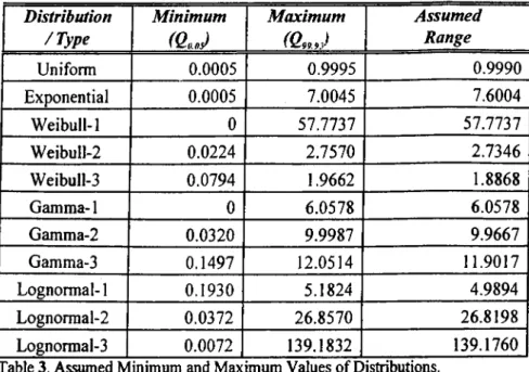
example, hence the set contains 23 rows. A difficulty arises in the preparation o f this

training set while trying to scale the quantile values to 0-1 range. Since most o f the

distributions considered are unbounded, there is the necessity o f assuming a finite range for

each distribution in order to be able to scale the absolute théorie quantile values with

respect to this interval. For this purpose an assumption is made by taking the values for

^ 0 0 5

and 109995 as the minimum and maximum values for each distribution. That means

0.05 percent probability is neglected from both tails o f the distributions and the finite range

is assumed to be

{ Q g g s s - Q ^ ) ·

Th^ same procedure is also applied to bounded

distributions in order to provide consistency among the distributions considered. These

values for each o f the 23 distributions are given in Table 3 below.

Distribution

/T ype

Minimum

( Q .J

Maximum

( Q „ J

Assumed

Range

Uniform

0.0005

0.9995

0.9990

Exponential

0.0005

7.0045

7.6004

Weibull-1

0 57.7737

57.7737

Weibull-2

0.0224

2.7570

2.7346

Weibull-3

0.0794

1.9662

1.8868

Gamma-1

0 6.0578

6.0578

Gamma-2

0.0320

9 . 9 m

9.9667

Gamma-3

0.1497

12.0514

11.9017

Lognormal-1

0.1930

5.1824

4.9894

Lognormal-2

0.0372

26.8570

26.8198

LognormaI-3

0.0072

139.1832

139.1760

(24)

Table 3(continued). Assumed Minimum and Maximum Values o f Distributions.

Distribution

/Type

Normal

B eta-1

Beta-2

Beta-3

Beta-4

Beta-5

Beta-6

Beta-7

Beta-8

Beta-9

B eta-10

B eta-11

Minimum

(QoJ

-3.2905

0.0015

0.0024

0.1822

0.0617

0.0376

0.0884

0.0130

0 0.0003

0.0263

0.0224

Maximum

(Q „ J

3.2905

0.8179

0.9384

0.9986

0.9977

0.9625

0.9117

0.9871

0.9737

0.9777

0.9998

Assumed

Range

6.5810

0.8164

0.9360

0.8164

0.9360

0.9249

0.8233

0.9741

0.9737

0.9774

0.9737

0.9774

The same range values are used to find the cumulative probability points o f interest.

For exam ple, for the case o f Beta-1, the cumulative probability at 0.4082 (midpoint o f

above range) is taken as

value in the training set.

The théorie skewness value for the Lognormal-3 distribution is changed to 13

instead o f 33.5 since our experience on empirical data revealed that the estimated skewness

has never been in the order o f 30, it varied around 13 even for a very large sample size like

2000

.

(25)

Chapter 4. Setting

₁₆

4.3 Probabilistic Neural Network (PNN)

The probabilistic neural network provides a general technique for solving pattern

classification problems. The PNN uses the training data to develop distribution functions

which are used to estimate the likelihood o f an input vector (feature vector) being within

the given categories.

PNN is a neural network implementation o f Bayesian classifiers method which was

developed in the 1950’s followed by Perzen Estimators that were developed in order to

construct the probability density functions required by Bayes theory.

Parzen estimation is used to build the probability density function over the feature

space for each category. This allows computing the probability that a given input vector

lies within a given category. Then combining this information with the relative frequency

o f each category, the PNN selects the most likely category for a given feature vector.

PNN was developed and described by D. Specht (1988). Bayes Classifier method is

implemented by the network where the class dependent probability density fimctions are

approximated using a Parzen estimator. Since a Bayes classifier provides an optimum

approach to pattern classification in terms o f minimizing the expected risk, and since

Parzen estimators asymptotically approach the true underlying class density functions as

the number o f training samples increase, PNN provides a very general and powerful

classification paradigm when there is adequate data o f known classification.

Suppose a classification problem has

K

classes

c „ c ; , - , Q

and suppose that the data on which decisions are based is represented by an M-dimensional

feature vector

x =[ x^, x^, - , x^, y

Let

be the probability density functions o f the class populations, and let

(26)

Then the Bayes decision rule compares the

K

values

P x f X A ^ P j i

■

· -rPK/K (x)

(

6 )

and chooses the class corresponding to the highest value. Loss functions can also be

utilized, but the main point about the decision rule is to evaluate the multivariate class

probability density functions at the given feature vector and compare them.

The decision rule depends on knowing the class probability density functions.

M aking some assumptions about the PDFs yields some common classification paradigms.

For exam ple, the assumption in a two class problem that the two PDFs are Gaussian with

the same covariance matrices yields the Fisher Linear Discriminant. Dropping the

assumption o f identical covariance matrices yields the quadratic Bayes classifier.

The Parzen estimator is a non-parametric method o f estimating PDFs which makes

no assumption about the nature o f the distribution. The Parzen estimator is built up from a

set o f smaller parametric fimctions, typically Gaussian Multivariate functions. In essence, a

sm all Gaussian curve is found for each training vector, then the curves are added together

and smoothed.

The Parzen estimator used in the Probabilistic Neural Network is o f the form

/*W=

1

1 r 1 ^

N,

y=i

. (7)

for class

k

where

x^j

is the

f ’

training sample in class

k,

is the number o f training

sam ples in category

k,

and

(

j

=

g

{N^)

(^)

is a sm oothing parameter which must satisfy

lim

<

t

(A^.) = 0

(9)

and

lim

N

i

^

o

{N^) = '

x

>.

Af,-».®

(27)

Chapter 4. Setting

₁₈

o ( N , ) = aN;>’

(11)

where 6 is a constant between 0 and 1.

The exponential constituents o f Equation (7) are referred to as Parzen kernels. They can be

rewritten as

({lx’’

x-xjj)/2a^)

₍

₁₂

₎

I f in addition, all inputs to the classifier have norm 1, then (12) can be rewritten as

(13)

The term

x '

j'tst

tlot product o f the feature veetor to be classified, with a training

vector. Therefore i f a processing element has its ineoming weights set to the training

vector, the standard summation produces that dot product. If the transfer function o f the

processing elem ent is o f the form

((z -l)/o ^ )

(14)

then the processing element implements (12).

The probabilistic network has an input buffer, a normalizing layer which maps the

input feature vectors to vectors o f norm 1, a pattern layer w hose incoming weights

correspond to the set o f training vectors, a summation layer which sums the Parzen kernels

for each class, and a classification layer which chooses the class with the largest response

to the input. The structure o f a typical probabilistic network is given in Figure 4.

(28)

Counter propagation network constructs a mapping from a set o f input vectors

X

to

a set o f output vectors

Y

acting as a hetero-associative nearest-neighbor classifier. Suitable

applications include pattern classification, function approximation, statistical analysis and

data com pression.

When presented with a pattern, the trained network classifies that pattern into a

particular group by using a stored reference vector; the target pattern associated with the

reference vector is then output.

The input layer acts as a buffer. The network operation requires that all the input

vectors have the same length, so input

vectors are normalized to norm 1.

Counterpropagation combines two layers from different paradigms. The hidden layer is a

Kohonen layer, with competitive units that do unsupervised learning. The processing

elem ents in this layer compete such that the one with the highest output wins and is

activated.

W j ' = W j + a ( x - W j )

(15)

where

a

is the learning rate.

A s shown in Figure 5, this means that the vectors

W

w ill tend to rotate around the unit

Sphäre

until they are at the center o f those input vectors

X

that create a maximum output. In

vector form the output / o f the processing element (before competition) is

I = W X

(16)

Since the length o f both the weight vector

W

and the input vector A" are 1, Equation (16)

reduces to

(29)

Chapter 4. Setting

₂₀

x-w

unit sphere

Figure 5. Adjustment of Weights by the Kohonen Learning Rule.

The Kohonen layer measures the cosine o f the angle between the input vector

X

and the

w eight vector

fF.

The processing element with closest weight vector (smallest angle /) has

the liighest output and wins. As a consequence the processing elements in the competitive

layer adjust their weight vectors to divide the input space in approximate correspondance to

the frequency with which the inputs occur.

The top layer is the Grossberg layer, which is fully interconnected to the hidden

layer and is not competitive. Since the Kohonen layer produces only a single output, this

layer provides a w ay o f decoding that output into a meaningful output class. The Grossberg

layer is trained by the Widrow-Hoff learning rule.

(

₁₈

)

where

is the desired output.

Since only one output from the Kohonen layer is active at a time, the only weight

adjusted for processing element /', is the one connected to the winning processing element^

in the com petitive layer. In this way the output layer learns to reproduce a certain pattern

for each active processing element in the competitive layer.

(30)

Different architectures for PNN and counter propagation networks are used. Also

architectures vary depending on the number o f training examples (for PNN) and on the

structure o f the training set used.

PNN consists o f 5 layers. There are 21 nodes in the input layer for training sets

containing all the skewness, quantile and cumulative probability information. Number o f

nodes for training sets which do not contain quantiles is 13. follow ing the input layer, there

is the normalizing layer which has no role in the laeming process, but acts as a buffer

which normalizes the inputs before entering the network.

The number o f processing elements in the pattern layer varies according to the

number o f examples in the training set used. Since each node in the pattern layer

corresponds to an example vector, there are 115 nodes for empirical training sets generated

from sam ples o f size 500, 1000 and 2000. In the case o f théorie training set, number o f

nodes is 23. For the mixed set combining all the training data (both empirical and théorie),

there are 368 nodes in this layer.

The number o f nodes in the summation and classification layers is equal to the

number o f categories to be classified, which is 23.

The nodes in the normalizing and pattern layers are fiilly interconnected with each

other. There is a special geometry o f connection between the summation and pattern layers.

The nodes in the pattern layer form groups and each group is connected to only one node in

the summation layer. Finally, there is a one-to-one connection between the summation and

classification layers.

The counter propagation networks used have 4 layers. A s in the case o f PNN, there

is an input layer consisted o f 21 or 13 nodes depending on the training set used, and a

normalization layer. The Kohonen layer has 35 nodes. The number o f nodes in the

hidden(Kohonen) layer is crucial for the counter propagation network because network

m em orizes (can not make good generalizations) when there is excess number o f nodes. On

the other hand the network may fail to learn if the number o f nodes is too few. The size o f

the hidden layer is determined by trial-and-error. There are 23 nodes in the Grossberg layer

corresponding to 23 categories. All nodes o f the network are fully interconnected.

(31)

Chapter 4. Setting

₂₂

4.6 Training the Networks

Networks are developed and trained by using the NWORKS Professional II

(NeuralWare Inc.-199I) software package.

Although at first, the coefficient o f kurtosis was included in the training sets, the

preliminary results indicated that it did not give useful information in detecting the

distributions. A lso the very large values o f kurtosis for the lognormal distributions (up to

the order o f 10000) caused a misleading effect while training the networks. Therefore, the

kurtosis is omitted from the training sets in further steps.

Similarly, the quantile values in the empirical training sets caused the networks fail

to leam. This is due to the requirement that the quantile values had to be scaled to 0-1

range in order to make them comparable among distributions. The range used for this

scaling purpose varied considerably for the empirical data, leading to different quantile

values for the same distribution. Consequently the empirical training sets are reconstructed

by omitting the quantiles and leaving the skewness and cumulative probability values. The

théorie training sets with quantile values did not cause training difficulties and both the

PNN and coimter propagation networks learned all the samples they were presented.

Three PN N s based on empirical training sets o f different sample sizes (500, 1000

and 2000) are trained by using the skewness and cumulative probabilities. The training

process took a very short time since just one pass o f the examples is required for the

training o f the PNN. In order to be able to compare the empirically trained networks with

the one trained with théorie data, another probabilistic network is trained by using a

training set which did not contain quantiles. Then an additional PNN is trained, this time

by using a combined training set which contained all the 3 empirical and the théorie data

sets. Totally there are six PNNs trained, three o f which are with empirical data (samples o f

size 500, 1000 and 2000 - containing no quantile), 2 with théorie data (one with quantiles

and other without) and one with mixed data (all empirical and théorie sets - again without

quantiles).

The attempts to train counter propagation networks with empirical training sets

showed that the output error term did not converge meaning that the networks were unable

to leam. Therefore counter propagation networks could be trained with théorie training sets

(32)

prepared exam ples in the sense that the examples from the categories to be distinguished

should be distinct and w ell defined without major similarities or overlaps among

categories. How ever this condition can not be satisfied with empirical training sets due to

the estimations performed during the preparation process.

A s a result, tw o counter propagation networks were trained with théorie data (one

with quantiles and other without) and learned all the categories. The training took about

6000 iterations and the root mean square (RMS) error converged almost to zero falling

below the level 1 e-5. The possible minimum number o f processing elements were used in

order to train the networks so as to enable the trained network to make correct

generalizations. For this purpose, starting with an initial number o f 30, the number o f

nodes in the hidden layer was incremented until the networks were able to leam all the

categories.

(33)

Chapter 5 RESULTS

After having trained the networks, the performance o f the learned networks is tested

by other data sets o f different sample sizes. For this purpose, 7 recall sets o f sample size

25, 50, 75, 100, 500, 1000 and 2000 were generated. Each recall set is composed o f 115

san ^ le vectors - 5 for each o f the 23 distributions/types. The recall sets were constructed

from raw data by using the same computer program employed for forming the empirical

training sets. There are two versions o f recall sets for each sample size - with and without

quantile values. The recall sets used for test purposes are given in tables AD1-AD7 in

Appendix D.

Each o f the eight trained networks was tested by using all the seven recall sets. The

networks’ output for a given recall set is a row o f 23 numbers for each input vector in the

test data. In order to provide a useful interface, a PASCAL program called “Evaluate” is

devdoped w hich process the output o f the network and prepare a performance report. By

using this program, the test input and the associated output o f the network, can be

examined together with the data used in the training stage, making it possible to get insight

aboBt the networks by achieving a comparative report on the mis classified items. The

program also creates a log file for convenience. The source code for this program is listed

in v^pendix B . Example log file showing the output o f this program is given in Appendix

C. The performance o f the networks is evaluated in two parts. In the first part, all the

23 different distributions/types are regarded as distinct. For example, a response by the

network recommending that a data set is from Weibull-2 category is treated as a false

choice i f the true underlying density that the data is generated from is Weibull-1 or

Weibull-3. In the second part, such an example is regarded as correct. In other words, the

network is accepted successful when it was able to tell the true distribution, even it could

not correctly decide on the specific type defined by the different shape parameter. Although

the trae underlying distributions o f the test data sets are known, especially for small sample

sizes it is probable that more than one distribution fits the data. To detect such cases, the

responds o f the networks are verified by the Chi-Square goodness o f fit test with a=0.05.

(34)

tabulates the values obtained by the first point o f evaluation and Table 5 shows the

performance o f the network in detecting only the density itself without the correct type.

Similarly the same procedure is applied for counter propagation networks. The results are

given in Tables 6 and 7. Also the performance o f the networks with different sample sizes

is graphed in Figures 6 and 7 for PNNs and in Figures 8 and 9 for counter propagation

networks.

The results indicate that, the probabilistic network performs better than the counter

propagation network in all the cases. Moreover, the performance o f the networks improve

when the sample size is increased. The performance o f the probabilistic networks in

identifying the correct type is about 50% for small sample sizes. When the restriction o f

identifying the correct type is released, the probabilistic networks’ performance jumps to

an acceptable level o f about 80% even for small samples o f size 25. It can be seen that the

quantile information did not contribute too much to the results, when w e compare the

performance o f the networks “théorie” and “quantile-theoric” in Tables 4 and 5. The

maximum improvement by adding the quantile information is achieved for small samples.

The effect gradually decreases when sample size gets larger. It can also be concluded that

regardless o f the training data set used, all the probabilistic networks performed more or

less identical.

The results for the counter propagation network indicate that although the network

learns the théorie data presented to it, it is not very successful in identifying new test

samples. When w e examine the actual results given by the network, w e see that most o f the

time when the network is hesitant between two or more candidate distributions, the output

is scattered (network distributes the output equally to all categories rather than deciding on

a single outcom e). This situation results from the structure o f the counter propagation

network. The output Grossberg layer, unlike the probabilistic network, is not organized as

competitive units. Therefore the network can remain hesitant among various choices.

However, in the PNN case, it is assured that only one processing element in the summation

layer with the highest output wins the competition and gets activated. Therefore it is

guaranteed that the network makes a choice.

(35)

Chapter 5. Results

26 A s stated before, another reason for the counter propagation network to fail is the

fact that counter propagation networks are devised for classification purposes when the

c a th o d e s are w ell separated. There are very similar distributions like Weibull-2, Weibull-

3, Gamma-2 and Gamma-3 or Normal and Beta-5 (see Figure 3) considered in this study,