Input data analysis using neural networks

128

TECHNICAL ARTICLE

Input

Data

_Analysis

Using

Neural Networks

Anil Yilmaz

Turkish Prime

_Ministry

State

_{Planning Organisation}

Yucetepe,

Ankara

_06100,

_Turkey

E-mail:

_{anil@dpt.gov.tr}

Ihsan

_Sabuncuoglu

Department

of Industrial

_Engineering

Bilkent

_University

Bilkent,

Ankara

_06533,

_Turkey

E-mail: sabun@bilkent.edu.tr

Simulation deals with

_{real-life phenomena by}

constructing representative

models

_{of a}

_system

being questioned. Input

data

_provide

a

_driving

force for

such models. The

_{requirement for}

iden-tifying

the

_underlying

distributions

_{of data}

sets

is encountered in

_{many fields}

and simulation

applications

(e.g., manufacturing

economics,

etc.). Most

_of

the _time,

_after

the collection

_of

the

raw

_data,

the true statistical distribution is

sought by

the aid

_of

_{nonparametric}

statistical methods. In _{this paper,} we

_investigate

_the

feasi-1. Introduction

z

Simulation models have a _{very wide range} of

applica-tion areas from

_{manufacturing}

to

defense,

economic and financial

_systems,

and the

_input

data used in these models are

_{usually represented by probability}

distri-bution functions. Since

_input

data

_provides

a

_driving

force for simulation

models,

this

_topic

is

_extensively

studied in the simulation literature

[1].

As also indi-cated

_by

Law and Kelton

_[2],

failure to choose the

cor-rect distribution can affect

_credibility

of simulation

models.

_However,

identification of the true

dif-distribution

_by

the aid of

_{nonparametric}

statistical methods

_(heuristics

and other

_graphical

_methods).

Summary

statistics such as _{minimum, maximum,}

mean,

median,

variance, coefficient of _variation, lexis

ratio, skewness, kurtosis,

etc., are

used,

as well as

other statistical

tools,

some of which are

_histograms,

line

_{graphs, quantile}

_summaries, box

_plots,

_Q-Q

and P-P

_plots.

In

_practice,

this task is sometimes

cumber-some and time

_consuming.

The aim of this

_study

is to

_investigate

the

_feasibility

of

_using

neural networks for the

_input

data

_analysis

(identification

of

_probability

_{distributions)}

and discuss the difficulties in

_using

neural

_networks,

as well as their

strength

and weaknesses over the traditional methods

(i.e.,

Chi-square goodness-of-fit

test,

etc.).

The rest _{of the paper} is

_organized

as follows. In

Sec-tion 2, we

_present

a brief review of the relevant litera-ture on the

_application

of neural networks to the

in-put

data

_analysis.

In Section 3, we

explain

the

method-ology

used in our

_study.

We

_give

the

_experimental

settings

in Section 4. The

_{computational}

results are

discussed in Section 5.

_Finally,

we make

concluding

remarks and

_suggest

further research directions.

2. Literature

_Survey

The

_input

data

_analysis,

which is also referred to as

input

data

_modelling

or

modelling

_input

_processes, is

not

_extensively

studied in the simulation literature. The

_topic

is discussed in detail in

_{[1], [2]}

and

_[3].

Gen-eral

_procedures

to

_identify

the correct distribution functions are also outlined in these references. In the

input

data

_analysis

literature,

Shanker and Kelton

[5]

investigated

the effect of distribution selection on the

validity

of

_output

from

_single

_queuing

models. The

. authors also

compared

the

_empirical

distribution functions

_(i.e.,

distribution of the

_sample

_data)

with standard

_parametric

distribution functions

_(e.g.,

Uni-form,

_Exponential,

Weibull).

Their results indicated that on the basis of variance and bias in their

estima-tions, the

_performance

of the

_empirical

distributions is

comparable

with,

even sometimes better

than,

standard distribution functions. Vincent and Law

_[6]

_proposed

a software

_package

called UNIFIT II for

_input

data

analysis.

The authors discuss the role of simulation

input

modeling

in a successful simulation

_study.

In a

related

_work,

Vincent and Kelton

_[7]

_investigated

the

importance

of

_input

data selection on

_validity

of

simu-lation models and discuss the

_{philosophical}

_aspects

of

the current

_thinking.

_Johnson

and

_Mollaghasemi

_[8]

explored

the

_topic

from a statistical

_point

of view. The authors

_provided

a

_{comprehensive bibliography}

and

a list of

_specific

research

_problems

in the

_input

data

analysis. Finally,

Banks, Gibson,

Mauer and Keller

[9]

discussed

_empirical

versus thoretical distributions and

_expressed

their

_opposite

views

_(points

and

coun-terpoints)

on

_input

data

_analysis.

In the neural network

literature,

neural networks

can be used in

place

of statistical

_approaches

_applied

to classification and

_prediction

_problems

_[10].

In

gen-eral,

_advantages

of neural networks in statistical

ap-plications

are their

_ability

to

_classify

robustness to

probability

distribution

_assumptions,

and the

_ability

to

_give

reliable results even with

_incomplete

data. In

this _context, neural networks are

_employed

where

re-gression,

discriminant

_{analysis, logistic}

_regression

or

forecasting approaches

are used.

Marquez

[11]

has

_provided

a

_complete

_comparison

of neural networks and

_{regression analysis.}

The results of his

_study

_suggest

that the neural networks can do

fairly

well in

_comparison

to

_regression

_analysis.

The

prediction

capability

of neural networks has been stud-ied

_by

a

_large

number of researchers. In

_early

_papers,

Lapeds

and Farber

_[12]

and Sutton

_[13]

offered evi-dence that the neural models are able to

_predict

time series data

_fairly

well.

_{Many comparisons}

of neural

networks and time series

_{forecasting techniques,}

such

as the

_Box-Jenkins

_approach,

are

_reported

_[10].

The

reader can refer to

_{[14], [15]}

and

_[16]

for further

read-ing

on

_application

of neural networks to data

_analysis.

In the

literature,

there are

_only

a few studies on the

application

of neural networks to the

_input

data

anal-ysis

problem

(Table 1).

The first

_study

in this area is

_by

Sabuncuoglu,

Yilmaz and

_Oskaylar

_[17],

who

investi-gated

the

_{potential applications}

of neural networks Table 1. A list of

_previous

studies and their characteristics

during

the

_input

data

_analysis

_stage

of simulation studies.

_{Specifically,}

_{counter-propagation}

and

back-propagation

networks were used as the

_pattern

classi-fier to

_distinguish

data sets _{among three basic} distri-bution functions:

_exponential,

uniform and normal.

Histograms

consisting

of ten

_equal-width

intervals

were used as

_input

vectors in the

_training

set. _The

per-formance of the networks was

compared

to the

stan-dard

_{goodness-of-fit}

tests for different

_sample

sizes and

_parameters.

The results indicated that neural net-works are

_quite

successful for identification of these three distribution functions.

Akbay,

Ruchti and Carlson

_[18]

_proposed

a neural

network

model,

which is based on the

_quantile

infor-mation to

_recognize

certain

_patterns

in raw data sets. The authors measured the

_{prediction capability}

of a

probabilistic

and a

_{back-propagation}

neural network

and

_compared

the results with traditional statistical

methods. Nine

_equal

interval normalized

_quantile

values were used as the

_input,

and 25 different

cat-egories

of distributions were identified. The results

indicated that the

_{probabilistic}

neural network

_(PNN)

learned

_(i.e.,

was able to

_{correctly identify)}

all the 25

categories

in the

_training

set, whereas the

back-propa-gation

network was able to learn 24

_categories.

In another

_{study, Aydin}

and

Ozkan

_[19],

_using

a

multi-layer

perceptron

network,

investigated

the per-formance of the neural network for

_{distinguishing}

among

normal,

gamma,

exponential

and beta distri-butions.

_{They compared}

the results with those of the

chi-square

test. The

_input

used for

_training

the net-works was selected as the minimum and maximum

values for the

distributions,

as well as normalized

fre-quencies.

The number of

_frequency

intervals to be used

was determined

_by

_constructing

various networks

with different numbers of

_frequency

intervals.

In a recent

_study,

Yilmaz and

_Sabuncuoglu

_[20]

de-veloped

a PNN to

_distinguish

23 different

_types

of

seven

_probability

distributions. The authors used

skewness,

_{eight quantile}

and twelve cumulative

prob-ability

values to train the neural network. Their results showed that PNN is

_good

at

_{hypothesizing}

the distri-bution of raw data sets. The authors also

_suggested

that there should be a

_grouping

of distributions with

similar

_shapes

and a

specialized

neural network should

implement

the selection process within each group.

30% reduction in the error

compared

to the best indi-vidual classifier. In another

_study,

_Jordan

and

_Jacobs

[23]

proposed

an

architecture,

which is a hierarchical

mixture model of

_experts

and

_expectation

maximiza-tion

_algorithms.

_By

this

_approach,

the authors divided

a

_{complex problem}

into

_{simpler problems}

that can be

solved

_by

_separate

_expert

networks. Boers and

_Kuiper

[24]

developed

a

_computer

_program to find a modular

artificial neural network for a number of

_application

areas

_(handwritten

_digit

_{recognition, mapping}

prob-lem,

etc.).

In a later

work,

Hashem

[25]

extended the

idea of

_optimal

linear combinations of neural networks and derive closed form

_expressions.

The results

dem-onstrated considerable

_improvements

in model

accu-racy,

leading

to a 81 % to 94% reduction in true MSE

compared

to the

_apparent

best neural network. The author also

_provided

a

_{comprehensive}

_bibliography

on

multiple

neural networks.

Yang

and

_Chang

_[26]

_proposed

a

_two-phase

learn-ing

modular neural network architecture to transform

a multimodal distribution into known and more

learn-able distributions.

_{They decomposed}

the

_input

_space

into several

_subspaces

and trained a

_separate

multi-layer

perceptron

for each group. A

_global

classifier network is trained for the second

_phase

of

_learning.

This network uses the

_inputs

from various local

net-works and maps this new data set to a final

classifica-tion _{space. The authors concluded that the}

_two-phase

learning

modular network architecture reduces to a

great

extent the chance of

_sticking

to a local minimum.

They

also argue that the

_two-phase

method is better

in

_performance

and more

robust,

and less

dependent

on architecture

_parameters

as well as selection of

training

samples.

’

Chen et al.

_[27]

_presented

a

self-generating

modu-lar neural network architecture to

_implement

the

di-vide-and-conquer

principle.

A tree-structured modular neural network is

_{automatically generated by}

recur-sively

partitioning

the

_input

_space. The results on

sev-eral

_{problems, compared}

to a

_{single multi-layer}

percep-tron, indicated that the

_proposed

method

_performs

well both in terms of

_high

success rate and short CPU time.

3. Research

_Methodology

We aim at

_{differentiating}

_among 23 different

_special

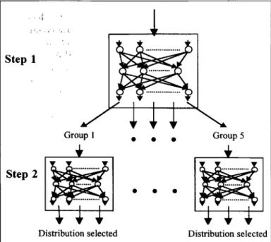
of distinct distributions based different

Figure

1.

_Two-step

_multiple

neural network

_approach

for

_multiple

neural networks.

According

to this

_approach,

in the first

_step

a

_single

network is used to

_classify

distributions with similar

shapes.

In the second

_step,

_specialized

networks are

used to detect different

_types

_{from each group of} dis-tribution functions. In _{this paper} we

_implement

this

two-step

multiple

neural network

_{approach (Figure}

_1).

Step

1 consists of

_grouping

distributions that have simi-lar

_shapes

and

_training

a neural network that

_performs

the classification task based on this

_grouping.

_Here, the

trained neural network is

_expected

to

_correctly

cat-egorize

among the different groups of distributions.

In the second

_step,

_{for each group of distributions} identified in the

_previous

_step,

a different network is

trained and tested. These

_specialized

networks are used

to further

_classify

the

_input

data into

_specific

distribu-tion functions. At this

_stage,

the

_training

sets and net-work structures _{for each group} are formed

_by

trial and error. The

_inputs

that would be most

_appropriate

for

each group are selected among all

_possible

_summary

statistics such as _range, mean, variance, coefficient of

variation,

skewness, kurtosis,

quantile

and cumulative

probability

information. In

_addition,

_composite

mea-sures such as kurtosis divided

_by

the coefficient of

variation or

_(skewness

+

_{kurtosis) /}

_(coefficient

of

variation)

are used in the

_experiments.

This selection

process is

explained

in detail in the

following

section. After

_training

the neural

_networks,

their

perfor-mances are measured

_by

_randomly

_generated

data of

known distributions. 4.

_Experimental

_Setting

4.1 Distributions Considered

There are seven distinct distributions used in this

study:

Uniform,

Exponential,

Weibull, Gamma,

Log-normal,

Normal and Beta. These distributions are

se-lected because

_they

are

_frequently

encountered in

sci-entific literature and real-life

_{applications.}

Based on

the different

_shape

_parameters,

we use three

_types

of

Weibull,

Gamma and

_Lognormal

distributions.

Simi-larly,

eleven different

_types

of Beta distribution are

considered

_{corresponding}

to different

_shape

param-eters.

_Totally,

23 distributions are used in the

experi-ments

_{(Table 2).}

4.2. Neural Network

_Types

and Structures

We

_initially

consider three neural network

_types:

back-propagation, counter-propagation

and

_{probabilistic}

neural networks

_[28].

Based on extensive

computa-tional

_experiments,

_however,

we eliminated the

back-propagation

and

_{probabilistic}

neural networks due to

their inferior

_performance.

Hence,

we

_mainly

focus on

the

_{counter-propagation}

network.

A

_{counter-propagation}

network constructs a

map-ping

from a set of

_input

vectors to a set of

_output

vec-tors

_acting

as a hetero-associative

_{nearest-neighbour}

classifier

_[29].

Its

_applications

include

_pattern

classifi-cation, function

_{approximation,}

statistical

_analysis

and data

_compression.

When

_presented

with a

_pattern,

the trained

counter-propagation

network classifies that

_pattern

into a

particular

group

by

using

a stored reference vector;

the

_{target pattern}

associated with the reference vector

is then

_output.

The

_input

_layer

acts as a buffer. The

network

_operation

_requires

that all the

_input

vectors

have the same

_length,

and hence

_input

vectors are

normalized to one. As discussed in

[30],

counter-propagation

combines two

_layers

_{from different}

para-digms.

The hidden

_layer

is a Kohonen

_layer,

with

competitive

units that

_{perform unsupervised}

learn-ing.

The

_processing

elements in this

_layer

_compete

such that the one with the

_highest

_output

is activated. The

_top

_layer

is the

_{Grossberg layer,}

which is

_fully

interconnected to the hidden

_layer.

Since the Kohonen

layer produces only

a

_single

_output,

this

_layer

pro-vides a _{way of}

_decoding

that

_output

into a

_meaningful

output

class. The

_{Grossberg layer}

is trained

_by

the Widrow-Hoff

_learning

rule.

4.3 Network _{Construction,}

_Training

and

_Testing

As discussed in the

_previous

_section,

the work is

car-ried out in two consecutive

_steps.

Step

1

_(Grouping

the _{Distributions):}

The distribution functions

_(given

in Table

₂₎

are

grouped

into six

_categories

based on their

_shapes.

The

clustering techniques

or

_unsupervised

neural networks

could have been used for

_grouping,

we

performed

this

step

manually.

First,

we formed

_preliminary

_groups

visually by

considering

their

_{general shapes (e.g.,}

Group

1

_represents

_bell-shaped

_{distributions,}

_Group

2 consists of

_right-skewed

_{distributions,}

_etc.).

Then we

looked at

_{skewness, kurtosis,}

_quantiles

and cumula-tive

_{probabilities}

of these distributions and finalized the

_grouping.

As can be seen in

_Appendix

1, skewness

and

_quantiles

of _{the different groups differ from each}

other,

whereas the distributions in each _group have

very close

parameters

values.

After

_forming

_{the above groups, the}

_training

set is

prepared.

For this _purpose, we use the UNIFIT-2

Sta-tistics

_Package

_[31].

All the

_possible

theoretical

sum-mary statistics for each of the 23 distributions are

in-vestigated

on the

_experimental

basis in order to find the

_inputs

that are useful for the network to

_distinguish

among groups. After numerous

_experiments,

skew-ness and

_quantile

information

_(measured

at seven

dif-ferent

_points)

are found to be the best

_{characterizing}

statistics. The

_training

set is

_given

in

_Appendix

1. Note

that some distributions in these groups are

duplicated

to form

_equal-size

_groups.

Hence,

equal

numbers of

examples

are

_presented

to the network to achieve a

balanced

_training.

The

_{proposed counter-propagation}

network has

eight

neurons

_{corresponding}

to

_eight

_inputs

in the

in-put

layer.

To determine the number of neurons in the

hidden

_{(or Kohonen)}

_layer

is a difficult task and is

usually

done

_by

_{experimentation.}

When there are too

many neurons, the network

memorizes,

and its

_ability

to

_generalize

_gets

weaker. On the other

hand,

using

too few neurons causes the network not to learn. Af-ter

_carrying

out some

_experiments

and

_considering

the above concerns, the number of

_processing

units in

the Kohonen

_layer

is determined to be fifteen. There

are six neurons in the

_{output (or}

_{Grossberg) layer}

cor-responding

to six _{groups of} distributions.

The

_{counter-propagation}

network is

_successfully

trained

_(i.e.,

the root mean _square

_(RMS)

error

con-verged

to

_zero)

_by

_using

the

_training

set

_given

in

Ap-pendix

1.

_{Specifically,}

it learned all the

_examples

in

the

_training

set after

5,000

iterations. In order to test the network

_performance,

a test set is

_prepared.

For

each of the 23

distributions,

five raw data sets of

sample

size 100 are

randomly generated.

The

result-ing

115 data sets are

processed by

a Pascal program

and are transformed into test

_examples,

each

repre-sented

_by

one skewness and seven

quantile

values.

When the test set is

_presented

to the trained neural

network,

it is observed that almost all test

_examples

are

_correctly

identified. The network fails for

only

three out of 115

_examples.

Hence, at this

_stage,

we

concluded that

_Step

1 of the

_{proposed procedure}

is

successfully

implemented.

Step

2 (Identification of Distributions):

In the second

_step,

we train a different neural net-work for five groups.

(Since

the sixth _group is uniform

itself,

there is no need to train a

_network)

Each group has its own attributes

_{(characteristics).}

Therefore,

_identifying

different distributions within each _group necessitates the use of different

_input

rep-resentation for each network. The

_inputs

that are most

suitable for each of the five _groups are identified

ex-perimentally

in the same _way as discussed in

_Step

1.

The

_training

set for each of _{the five groups} is

_given

in

Appendix

2.

The

_topology

of the

_{counter-propagation}

network

varies _{among groups. The number of}

_input

_layer

neu-rons is determined

_by

the number of

_inputs

in the

training

examples.

Also,

the number of neurons in the hidden

_layer

_{for each group} is found on the

experi-mental basis.

Here,

we observed that it would be

suit-able to use twice as _many neurons as the number of

distributions to be identified in _{each group. The}

num-ber of

_output

neurons is determined

_by

the number of

distributions that form the _groups.

All the five neural networks are

_successfully

trained as the RMS errors _converge to zero after _5,000 itera-tions. The trained networks are tested

_by

the same

data sets

_generated

in

_Step

1.

_Again,

the raw data sets

are transformed into

_appropriate

test

_{examples by}

the Pascal

_computer

_{program. The results of the} tests are

discussed in detail in the next section.

5. Results

Having

trained the neural networks

_{successfully,}

we measure their

_{performances by}

the test data sets of

sample

size _{50, 100} and 500

_(a

total of 345 test

exam-ples).

In

_Step

_1, when the test data sets are

_presented

to

the trained

_{counter-propagation}

network,

it identified the correct

_grouping

with 97.4% success

_{(Table 3).}

All

the

_examples,

which

_belong

to

_Groups

_{1, 3, 5} and the

uniformly

distributed set

_(Group

_6),

were

_perfectly

categorized.

For

_Group

2, 24 out of 25 sets were

suc-cessfully

classified,

whereas the success rate was 13

out of 15 for

_Group

4.

In

_general,

we observed that the neural network

performance

improves

as

_sample

size increases

_(see

Table

_3).

It can also be noted that the success rate in

Step

1 is

_higher

than in

_Step

2. This is

_expected

because neural networks used in

_Step

2 have to

_distinguish

specific

distributions _among similar

distributions,

.

whereas the neural network used in

_Step

1

_just

classi-fies the _{distributions among} more distinct groups.

By examining

the results in Table

_3,

we can

con-clude that neural networks should not be

recom-mended for small

_sample

_sizes; the success rate of the

two-step

neural network

approach

is around 58% for

Table 3. Test results for the neural networks

I I

successful,

consist of

_mostly

beta distributions with different

_shape

_parameters.

_Group

6

_(uniform)

is also

a

special

_type

of beta distribution. This means that

neural networks are

_quite

successful in

_{distinguishing}

beta distributions. To some _{extent, the}

_ability

of the

neural networks to

_distinguish

the beta distribution from the others also continues for

_Group

1

(symmet-ric-bell

_type).

It seems that the second _{group which includes}

ex-ponential,

Weibull,

_Lognormal

and Gamma

distribu-tions, is the most _{difficult group for} our neural

net-work

_approach.

Note that this _group consists _{of very}

skewed distributions

_(skewed

to the

_right)

_which

ap-parently

created a

_great

deal of

_difficulty

for the

neu-ral model.

Results also indicated that the

_two-step

_multiple

neural network

_{approach proposed}

in _{this paper} is

more successful than the

_one-step

_single

neural net-work

_approach

discussed in

_[20].

As seen in Table

4,

the

_percentage

of

_improvement

by

the

_two-step

_approach

is lowest for small

_sample

sizes, moderate for

_{large sample}

sizes and

_highest

for

medium

_sample

size

_{(n = 100).}

The

_multiple

neural network

_{approach proposed}

in

this paper and traditional

_{goodness-of-fit}

tests

_(GFT)

are not

_{directly comparable,}

because the

_proposed

ap-proach

is a meta model which selects a distribution for

the

_given

data set

_(i.e.,

_rejects

all the other candidate distribution

_functions),

whereas GFT is more an

analy-sis tool which tests if a candidate distribution is a

_good

fit for the data set.

_{(This concept}

is illustrated in

Fig-ure 3 where Di

_represents

the i-th distribution function

and

_Si

_corresponds

to the i-th

_step

of the

_multiple

neu-ral network

_approach).

While

_doing

_that,

GFT

_might

require

more than one iteration for

_testing

candidate

distributions. It is also

_quite

_possible

that GFT

_might

reject

the true

_underlying

distributions. In our case, for

_example,

a

_{chi-square goodness-of-fit}

test

_applied

to data sets

_rejected

eleven and six distributions for

sample

sizes 50 and

_100,

_{respectively.}

This means that

this

_technique

is less reliable when the

_sample

size is

small.

Another

_{distinguishing}

characteristic of the neural network

_approach

from GFT is that once a distribution

is

selected,

other alternative distributions are

rejected.

Figure

3. ANN versus

_{goodness-of-fit}

tests

easily

pass the test in the classical GFT

approach.

Hence,

the results of the GFT test _may not

_always

be

conclu-sive. In that

_respect,

GFT and neural networks should

be considered as

_{complementary techniques.}

Specifi-cally,

the results of the neural network

_(i.e.,

distribu-tion recommended

_by

the neural

_network)

can be used

by

the GFT to make more reliable and

_quicker

decisions.

6.

_Concluding

Remarks

In this _paper, we

developed

a

_multiple

neural network

architecture to select

_probability

distribution functions. The results indicated that the

_multiple

neural network

approach

is more successful than the

_one-step

_single

neural network

_approach

in

_identifying

distributions.

In this

_study,

we also

_analysed

the

_strengths

and

weaknesses of neural networks relative to the tradi-tional GFT

_approach.

Our conclusion is that the

neu-ral networks can be

_successfully

used in simulation

input

data

_analysis

as a

_quick

reference model. In this

context, neural networks can

_complement

the function

of the traditional GFT

_approach

_(i.e.,

the

_suggested

reference models can be further

_analysed

_by

the

tradi-tional

_methods).

Even

_though

some

_groundwork

has been estab-lished in this _paper, there are several research issues that need to be addressed in future studies. _First,

neu-ral networks can be trained to act as a traditional GFT

(Figure

3(b)).

In this case, one

_special

neural network

is trained for each distribution function and is used to

accept

or

_reject

the

_hypothesis.

Second,

the

perfor-mance of the neural network

_approach

in this

prob-lem domain can be

_{improved by}

_using

different NN

architectures.

Third,

_unsupervised

neural networks

can be used to form the _groups.

_Finally,

neural net-works can be used in

_estimating

the

_parameters

of the

distributions. This may be a fruitful future research area for neural networks in the field of

_probability

distribution selection.

7. References

[1] Vincent, S.G. _"Input Data _Analysis." In Handbook _of

Simula-tion, J. Banks _{(ed.), pp} 55-91, 1998.

[2] Law, A. and Kelton, W.D. Simulation _Modeling and _Analysis,

Second Edition, McGraw-Hill, 1991.

[3] Banks, J., Carson, J.S. and Nelson, B.L. Discrete Event _System

Simulation, Second Edition, Prentice- Hall, 1996.

[4] Bratley P., Fox, B.L. and _Schrage, L.E. A Guide to Simulation,

Second Edition, Springer-Verlag, New York, 1987.

[5] Shanker A., and Kelton, W.D. _{"Empirical Input} Distributions:

An Alternative to Standard _Input Distributions in Simulation

Modeling." Proceedings of the 1991 Winter Simulation

Confer-ence, B.L. Nelson, W.D. Kelton and G.M. Clark (eds.), pp

978-985, 1991.

[6] Vincent, S.G. and Law, A.M. "Unifit II: Total _Support for Simulation Input Modelling." Proceedings of the 1992 Winter Simulation _{Conference, J.J. Swain,} D. Goldsman, R.C. Crain and J.R. Wilson (eds.), pp 136-142, 1991.

[7] Vincent, S.G. and Kelton, W.D. "Distribution Selection and

Validation." _{Proceedings of the} 1992 Winter Simulation

Confer-ence, J.J. Swain, D. Goldsman, R.C. Crain and _J.R. Wilson

(eds.), pp 300-304, 1992.

[8] Johnson, M.E. and _{Mollaghasemi,} M. "Simulation _Input Data Modelling." Annals _{of Operations} Research, Vol. 53, pp 47-75,

1994.

[9] Banks, J., Gibson, R.R., Mauer, J. and Keller, L. "Simulation

Input Data: _{Point-Counterpoint."} IIE _{Solutions, January 1998,}

pp 28-36, 1998.

[10] Sharda, R. "Neural Networks for the MS/OR _Analyst: An Ap-plication Bibliography." Interfaces, Vol. 24, pp 116-30, 1994.

[11] Marquez, L.O. "Function _{Approximation Using} Neural

Net-works : A Simulation _Study." PhD Dissertation, University of

Hawaii, Honolulu, HI, 1992.

[12] Lapeds, A. and Farber, R. "Nonlinear _Signal Prediction _Using

Neural Networks: Prediction and _{System Modeling."}

LA-UR-87-2662, Los Alamos National _Laboratory, Los Alamos,

NM, 1987.

[13] Sutton, R.S. _"Learning to Predict the Method of _Temporal

Differences." Machine _Learning, Vol. 3, No. 1, pp 9-44, 1988.

[14] Ali, D.L., Ali, S. and Ali, A.L. "Neural Nets for Geometric

Data Base Classifications." _{Proceedings of the} SCS Summer

Simulation _{Conference, pp} 886-890, 1988.

[15] Pham, D.T. and Oztemel, E. "Control Chart Pattern Recogni-tion _Using Neural Networks." Journal of Systems Engineering, Vol. 2, pp 256-262, 1992.

[16] Udo, G.J. and _Gupta, Y.P. _{"Applications} of Neural Networks

in _{Manufacturing Management Systems."} Production _Planning and Control, Vol. 5, No. 3, pp 258-270, 1994.

[17] Sabuncuoglu, I., Yilmaz, A. and _Oskaylar, E. _"Input Data

Analysis for Simulation _Using Neural Networks." In

Proceed-ings of the Advances in Simulation ’92 _Symposium, A.R. _Kaylan and T.I. Ören (eds.), pp 137-150, 1992.

[18] Akbay, K.S., Ruchti, T.L. and Carlson, L.A. _"Using Neural Net-works for _{Selecting Input Probability} Distributions."

Proceed-ings of ANNIE’92, 1992.

[19] Aydin, M.E. and Özkan, Y. _{"Da∂ylym} Türünün Belirlenmes-inde _Yapay Sinir _{A∂larynyn Kullanylmasy." Proceedings of} the

First Turkish _Symposium on _{Intelligent Manufacturing Systems,}

pp 176-184, 1996.

[20] Yilmaz, A. and _Sabuncuoglu, I. _"Probability Distribution Se-lection _Using Neural Networks." _{Proceedings of} the _European Simulation _{Multiconference} ’97, 1997.

[21] Hashem, S. and Schmeiser, B. _"Improving Model _Accuracy

Using Optimal Linear Combinations of Trained Neural

Net-works." IEEE Transactions on Neural Networks, Vol. 6, No. 3,

pp 792-794, 1995.

[22] Rogova G. _"Combining the Results of Several Neural Network Classifiers." Neural Networks, Vol. 7, No. 5, pp 777-781, 1994.

[23] Jordan, M.I. and Jacobs, R.A. "Hierarchical Mixtures of

Ex-perts and the EM _Algorithm." Neural _Computation, Vol. 6,

pp 181-214, 1994.

[24] Boers, E.J.W. and _Kuiper, H. _{"Biological Metaphors} and the

Design of Modular Artificial Neural Networks." Masters

Thesis, Departments of _Computer Science and _Experimental

and Theoretical _Psychology at Leiden _University, The

Neth-erlands, 1992.

[25] Hashem, S. _"Optimal Linear Combinations of Neural

Net-works." Neural Networks, Vol. 10, No. 4, pp 599-614, 1997.

[26] Yang, S. and _Chang, K. "Multimodal Pattern _{Recognition by} Modular Neural Network." _{Optical Engineering,} Vol. 37,

No. 2, pp 650-659, 1998.

[27] Chen, K., _Yang, L., Yu, X. and Chi, H. "A _{Self-Generating}

Modular Neural Network Architecture for _Supervised

Learning." Neurocomputing, Vol.16, pp 33-48, 1997.

[28] Bose, N.K. and _Liang, P. Neural Network Fundamentals with

Graphs, Algorithms, and _{Applications,} McGraw-Hill, 1996.

[29] NeuralWare, Inc. Neural _{Computing, Pittsburgh,} 1991.

[30] Hecht-Nielsen, R. _{Neurocomputing, Addison-Wesley,} 1990.

[31] Law, A. and Vincent, S.G. _Unifit II User’s Guide. Averill M. Law & Associates, Tucson, AZ, 1994.

Appendix

2:

_Training

Sets for

_Step

2 Anil Yilmaz is an _expert at the Turkish Prime

Ministry-Undersecretariat of the State

Plan-ning

Organization.

He received a

BSc

_degree

in Industrial

Engineer-ing

and an MA

_degree

in

Econom-ics from Bilkent

_University

in

Tur-key.

He has been associated with the

_planning

of

_public

investments,

project appraisal,

and investment

analysis

and

_monitoring.

Yilmaz is

currently

working

as the

Counsel-lor to the

_{Undersecretary.}

Ihsan

_Sabuncuoglu

is an Associate

Professor of Industrial

_Engineering

at Bilkent

_University.

He received

BS and MS

_degrees

in Industrial

En-gineering

from Middle East Techni-cal

_University

and a PhD in

Indus-trial

_Engineering

from Wichita State

University.

Dr.

_Sabuncuoglu

teaches and conducts research in the areas of neural networks,

simu-lation,

scheduling,

and

manufactur-ing

systems. He has

_published

pa-pers in l1E 1’ransactions, International

Journal

of

Production _{Research, Journal}

_of

_{Manufacturing}

Sys-tems, International _Journal

_of

Flexible

_{Manufacturing Systems,}

International

_Journal

_of

_{Computer Integrated}

_{Manufacturing,}

Computers

and

_Operations

Research,

European

Journal

of

Opera-tional Research, Production

_Planning

and _{Control, Journal}

_of

Operational

Research

_Society,

_Computers

and Industrial

Engi-neering,

International _Journal

_of

Production Economics,

journal

of Intelligent Manufacturing

and OMEGA-International

Jour-nal

_{of Management}

Sciences. He is on the Editorial Board of

Journal

of Operations Management

and International _Journal

_of

Operations

and _Quantitative

_Management.

He is an associate

member of Institute of Industrial

_Engineering

and Institute