Non-incremental classification learning algorithms based on voting feature intervals

ste·. й. ЙТІШІ ' I

.S.Î üıS® İÎ!^ Л?

jŞ y f.jfe jÎ J Ü L j i І£ і?й % Э bi-S’İ Î ':# w i J ı«<-a·.* .

N O N -IN C R E M E N T A L

C LA SSIFIC A TIO N L E A R N IN G

A LG O R ITH M S B A SED ON

V O T IN G F E A T U R E INTERVALS

by

Giil§en Demiroz

August, 1997

6 ·0

Gift ?é.e>

I certify that I have read this thesis and thcit in my opinion it is fully adecpiate, in scope and in quality, as a thesis for the degree of Master of Science.

v u T l

Assoc. Prof. Halit Altay Güvenir (Advisor)

I certify that I have read this thesis and that in my opinion it is fully cidequate, in scope and in quality, as a thesis for the degree of Master of Science.

Asst. Prof. Ilyas Çiçekli

I certify that I have read this thesis and that in my opinion it is fully adequate, in scope and in quality, as a thesis for the degree of Master of Science.

,jy L

Asst.Prof. Özgür Ulusoy u

Approved for the Institute of Engineering and Science:

Prof. Melimet Bar^

Director of Institute of Engineering and Science

A B S T R A C T

NON-INCREMENTAL CLASSIFICATION LEARNING

ALGORITHMS BASED ON VOTING FEATURE

INTERVALS

Gül§en Demiroz

M.S. in Computer Engineering and Information Science Supervisor: Assoc. Prof. Halil Altay Giivenir

August, 1997

Learning is one of the necessary abilities of an intelligent agent. This thesis proposes several learning algorithms for multi-concept descriptions in the form of feature intervals, called Voting Feature Intervals (VFI) algorithms. These algorithms are non-incremental classification learning algorithms, and use fea­ ture projection based knowledge representation for the classification knowledge induced from a set of preclassified e.xamples. The concept description learned is a set of intervals constructed separately for each feature. Each interval car­ ries classification information for all classes. The classification of an unseen instance is based on a \oting scheme, where each feature distributes its \o te among all classes. Empirical evaluation of the VFI algorithms have shown that they are the best performing algorithms among other prex iously developed fea­ ture projection based methods in terms of classification accuracy. In order to further improve the accuracy, genetic algorithms are developed to learn the op­ timum feature weights for any given classifier. Also a new crossover operator, called continuous uniform crossover, to be used in this weight learning genetic algorithm is proposed and developed during this thesis. Since the e.xplanation ability of a learning system is as much important as its accuracy, VFI classi­ fiers are supplemented with a facility to convey what the}^ have learned in a comprehensible way to humans.

K eyw ords: machine learning, supervised learning, classification, inductive learning, non-incremental learning, feature intervals, voting, genetic algorithms.

ÖZET

OYLAYAN ÖZNİTELİK BÖLÜNTÜLERİNE DAYALI

TOPLU SINIFLANDIRMA ÖĞRENME ALGORİTMALARI

Gülşen Demiröz

Bilgisayar ve Enformatik Mühendisliği, Yüksek Lisans Tez Yöneticisi: Doç. Dr. Halil Altay Güvenir

Ağustos, 1997

Öğrenmek akıllı bir bireyin en gerekli özelliklerinden biridir. Bu tezde çoklu kavram tanımlarını öznitelik aralıkları şeklinde öğrenen yeni algoritmalar öne­ rilmektedir. Oylayan Öznitelik Aralıkları (VFl) olarak isimlendirilen bu al­

goritmalar toplu sınıflandırma öğrenme algoritmalarıdırlar. Daha önceden

sınıflandırılmış olan örneklerden sınıflandırma bilgisini çıkarmak için öznitelik izdüşümlerine dayalı bilgi gösterim yöntemini kullanırlar. Öğrenilen kavram tanımı her öznitelik için ayrı ayrı öğrenilen aralıklar şeklindedir. Her bir aralık bütün sınıflar için sınıflandırma bilgisi içerir. Yeni bir örneğin sınıflandırılması her özniteliğin oyunu bütün sınıflara dağıttığı bir oylama, sistemine dayanır. Gerçek hayattan alınan veri kümeleri üzerinde yapılan deneylerde \ T I algo­ ritmaları daha önce geliştirilmiş öznitelik izdüşümlerine dayalı diğer metod- lardan daha yüksek sınıflandırma doğruluğu elde etmişlerdir. .Ayrıca sınıf­ landırma doğruluğunu daha çok arttırm ak için optimum öznitelik ağırlıklarını öğrenen genetik algoritmalar geliştirilmiştir. Aynı zamanda bu genetik algo­ ritmalarda kullanılmak üzere yeni bir çaprazlama operatörü de geliştirilmiştir. Bir öğrenme sisteminin açıklama yeteneği de en az doğruluğu kadar önemli olduğundan, VP'I algoritmaları öğrendiklerini insanların anlayabileceği bir şe­ kilde gösterebilmektedirler.

A n a h ta r Sözcükler: öğrenme, tümevarımsal öğrenme, sınıflandırma, toplu öğrenme, denetimli öğrenme, öznitelik izdüşümleri, oylama, genetik algorit­ malar.

ACKNOWLEDGMENTS

I would like to express my gratitude to Assoc. Prof. H. Altay Güvenir, from whom I have learned a lot, due to his supervision, suggestions, and un­ derstanding throughout the development of this thesis.

I am also indebted to Assist. Prof. Özgür Ulusoy and Assist. Prof. Ilyas Çiçekli for showing keen interest to the subject m atter and accepting to read and review this thesis.

I would like to thank to Halime Büyükyıldız for everything, Esra Erdem for her mails at any time from Texas, Gökmen Gök especially for his poems, my yoga friends, Antal van den Bosch for his friendship at the conferences. Serap Yılmaz, Bahtiser Kuş, Aynur Akkuş, Bilge Aydın, my sister Ayşen Demiröz, my vounger sisters, and my parents for their morale support and friendship. I should not forget to thank to the bars in .Ankara to which usually I and Halime were used to go.

1 would also like to thank Bilkent University, which enabled this research environment and supported the presentation of this work at conferences.

This thesis was supported by TUBITAK (Scientific and Technical Research C’ouncil of Turkey) under Grant EEEAG-153.

C o n ten ts

1 Introduction 1

2 Supervised Inductive Learning M odels 6

2.1 Exemplar-Based Learning 7

2.1.1 Instance-Based L e a rn in g ... 9

2.1.2 Nested-Generalized E xem plars... 11

2.1.3 Feature Projection Based L e a r n in g ... 14

2.2 The Nearest Neighbor C lassifier... 14

2.3 Decision T rees... 16

2.4 Naive Bayesian C lassifier... 21

3 Feature Projection Based Learning M odels 27 3.1 I\ Nearest Neighbor Classification on Feature Projections . . . . 28

3.2 Classification by Feature P a rtitio n in g ... 30

3.3 Feature Intervals Learning .Algorithms 34

3.4 Classification with Overlapping heature Intervals 37

4 Classification by Voting Feature Intervals 41

4.1 Basic Definitions ... 43

4.2 Description of the VFI Algorithms 46 4.2.1 The VF'll A lg o rith m ... 46

4.2.2 The VFI2 A lg o rith m ... 55

4.2.3 The VF13 A lg o rith m ... 57

4.2.4 The VT'14 .A lgorithm ... 63

4.2.5 The VF15 A lg o rith m ... 67

4.3 Characteristics of VTI A lgorithm s... 70

4.3.1 Knowledge R epresentation... 70

4.3.2 Supervised Inductive L earning... 71

4.3.3 Non-incremental (Batch) Learning 71 4.3.4 Domain Independence in Learning... 72

4.3.5 Multi-concept L earning... 73

4.3.6 Properties of Feature V alu es... 73

1.3.7 Handling Missing (Unknown) Feature V alues... 74

4.4 Implementation and User I n te r f a c e ... 74

4.5 Summary 78 5 Evaluation o f the V FI Algorithm s 80 5.1 Comple.xity .A n aly sis... 80

5.1.1 Space C'omplexity Analysis... 81

5.1.2 Time Complexity of Training 82

5.1.3 Time Complexity of a Single Classification... 83

5.2 Empirical Evaluation of the VFI Classifiers on Real-World Datasets 84 5.2.1 Testing M ethodology... 85

5.2.2 Experiments on Real-World D a ta s e ts ... 87

5.2.3 Experiments on Artificial Datasets 95 5.3 D iscussion... 105

6 Learning Feature W eights 107 6.1 Genetic A lgorithm s...109

6.2 Weight Learning Genetic A lg o rith m s...117

6.3 E xperim ents... 118

6.3.1 Weighted Nearest Neighbor C lassifier... 118

6.3.2 Weighted N oting Feature Intervals Classifiers... 120

6.4 Summary and Discussion... 122

7 V isualization of the Learned C oncepts 124

8 Conclusions and Future Work 141

A Real-W orld D atasets 155

List o f F igu res

2.1 Classification of Exemplar-Based Learning models. 8

2.2 An example concept description of the EACH algorithm in a domain with two features... 1.3 2.3 The Training in the NBC Algorithm.

2.4 The Classification in the NBC Algorithm.

23 24

2.5 Computing the a posteriori probabilities in the NBC Algorithm. 25

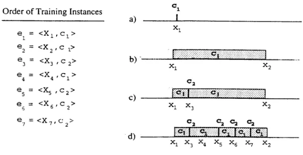
3.1 Construction of intervals in the CEP algorithm: (a) after ti is

processed, (b) after 62 is processed, (c) after 63 is processed, (d) after all training instances are processed... 31 3.2 Construction of intervals in the CF'P algorithm by changing the

order of the training instances. Note that here the same set of instances in Figure 3.1. but in a different order, is used as the

training set: (a) after €3, e·;. 65 and cq are processed, (b) after

all instances are processed. 33

3.3 Construction of the intervals in the FIL algorithms with using

the same dataset as used in Figure 3.1 and Figure 3.2. 36

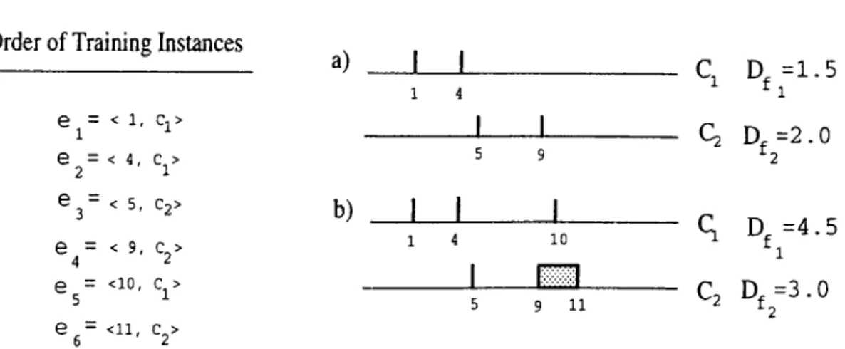
3.4 .An example of construction of intervals in the COFI algorithm:

(a) after fi. ( 2· ^3 and € 4 are processed, (b) after (5 and tn are

processed... 38

3.5 An example of construction of intervals in the COFI algorithm using the same set of training instances as in Figure 3.6, but in a different order: a) after e\. 65, 63, and eg are processed, b)

after t2 and £4 are processed. 40

4.1 An example for three intervals on a feature dimension

f.

4.2 An example for three point intervals on feature dimension color. 45

4.3 Training phase in the VFIl .Algorithm... 47 4.4 Classification in the VFIl Algorithm... 48

4.5 A sample training dataset with two features and two classes. . . 52

4.6 The constructed intervals by VFIl with their class counts for the sample dataset... 52 4.7 The constructed intervals by \ ’F I1 with their class votes for the

sample dataset... 53 4.8 The constructed intervals by \ ’FI1 with their class votes for the

training dataset in Figure 3.1... .54 4.9 The constructed intervals by \ ’F I1 with their class votes for the

training dataset in Figure 3.4... 55 4.10 Training phase in the VF12 .\lgorithm ... 56 4.11 The constructed intervals by \ FI2 with their class counts for

the sample dataset... 57 4.12 The constructed intervals by \ FI2 with their class votes for the

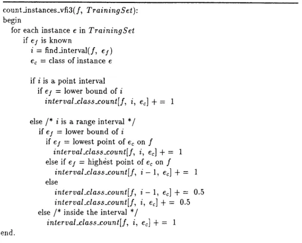
sample dataset... 57 4.13 The algorithm for counting the training instances in the training

phase of the VFI3 classifier. 59

4.14 Classification in the VFI3 Algorithm... 60

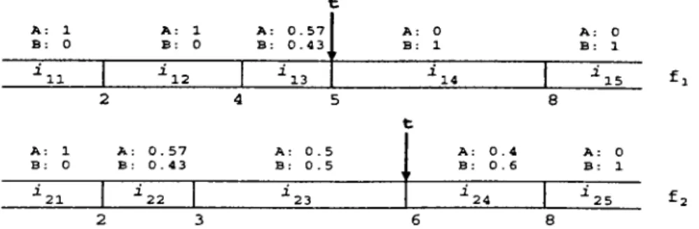
4.15 The constructed intervals by VFI3 with their class counts for the sample dataset... 61 4.16 The constructed intervals by VTI3 with their class votes for the

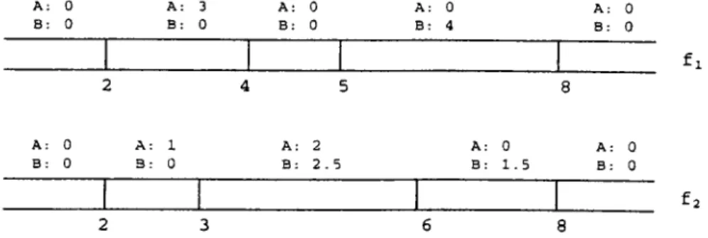
sample dataset... 61 4.17 The projection of a sample dataset with two classes on linear

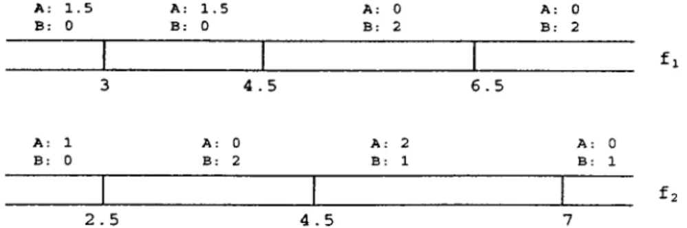
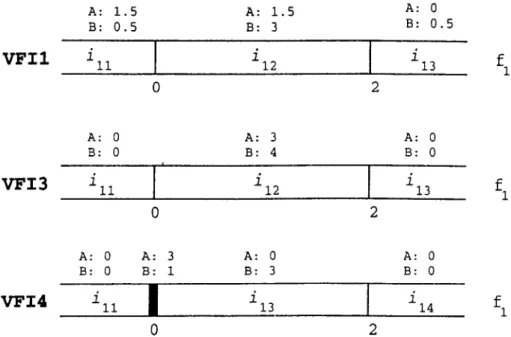
feature dimension / i ... 63 4.18 The constructed intervals by V FIl, VFI3, VFI4 with their class

counts for the second sample dataset... 63 4.19 Training phase in the VFI4 Algorithm... 65 4.20 Training phase in the VFI5 Algorithm... 68 4.21 The constructed intervals by VFI5 with their class counts for

the sample dataset... 68 4.22 The constructed intervals by VFI5 with their class votes for the

sample dataset... 69

4.23 .\n example for the information provided to the FIL algorithms. 74

4.24 The visualization of the feature intervals constructed by the VFI algorithms for the Dermatology dataset by our user interface.. . 76 4.25 The visualization of the feature intervals constructed by the VFI

algorithms for the .\rrhythmia dataset by our user interface. . . 77

5.1 The algorithm for .V-fold cross-validation... 86

5.2 .Average training time of all classifiers on datasets with increas­ ing number of instances. 9/10 of the whole dataset is used in training... 92 5.3 .Average training time of all \'F I versions on datasets with in­

creasing number of instances. 9/10 of the whole dataset is used

in training. 93

5.4 Average classification time of all classifiers on datasets with in­ creasing number of instances. 1/10 of the whole dataset is used in classification... 94 5.5 Average classification time of all classifiers except the 1-NN al­

gorithm on datasets with increasing number of instances. 1/10 of the whole dataset is used in classification... 94 5.6 Average classification time of all VFI versions on datasets with

increasing number of instances. 1/10 of the whole dataset is used in classification... 95 5.7 10-fold cross-validation accuracy results of the VFI algorithms

compared with that of CFP, COFI, 1-NNFP, and FI4 algorithms on Iris dataset with increasing number of irrelevant attributes. . 97 5.8 10-fold cross-validation accuracy results of the VFI algorithms

compared with that of 1-NN, C4.5, NBCN algorithms on Iris dataset with increasing number of irrelevant attributes... 97 5.9 10-fold cross-validation accuracy results of the VFI algorithms

compared with that of CFP, COFI, 1-NNFP, and FI4 algorithms on Iris dataset with increasing level of noise... 99 5.10 10-fold cross-validation accuracy results of the VF'I algorithms

compared with that of 1-NN, C4.5, NBCN algorithms on Iris dataset with increasing level of noise... 99 5.11 10-fold cross-validation accuracy results of the VFI algorithms

compared with those of CFP. COFI, 1-NNFP. and FI4 algo­ rithms on Iris dataset with increasing percentage of unknown values in training dataset... 102 5.12 10-fold cross-validation accuracy results of the VF'I algorithms

compared with those of 1-NN. NBCN, and C l.5 on Iris dataset with increasing percentage of unknown values in training dataset. 102

5.13 10-fold cross-validation accurac}· results of the VFI algorithms compared with those of CFP, COFI, 1-NNFP, and FI4 algo­ rithms on Iris dataset with increasing percentage of unknown values in test data... 10-1 5.14 10-fold cross-validation accuracy results of the VFI algorithms

compared with those of 1-NN, NBC.N, and C4.5 algorithms on Iris dataset with increasing level of unknown values in test data. 104

6.1 The algorithm for a genetic algorithm... 110

6.2 Algorithms for One-Point Crossover, Two-Point Crossover, and Uniform Crossover...113 6.3 The G.A-C7«.ss?^e?· Feature Weighting Algorithm...117 6.4 Comparison of IPCO-WNN, 2PCO-WNN, UCO-WNN, and CUCO-

WNN on real-world datasets for increasing number of genera­ tions. The accuracy results are obtained by .5-fold cross-validation. 121

7.1 Concept Description Learned by \ ’FI1 including only a feAv fea­

tures...126 7.2 Concept Description Learned by \TT2 including only a few fea­

tures... 127 7.3 Concept Description Learned by \'F I3 including only a few fea­

tures...129

7.1 Concept Description Learned by \ ’F14 including only a few fea­

tures... 130 7.5 Concept Description Learned by \ ’FI5 including only a few

lea-tures... 132 7.6 -'\ correct classification of a. given test instance (patient) drawn

from the Dermatology domain by the VFll classifier...13-1

7.7 Another correct (not that confident as the previous classifica­ tion) classification of a given test instance (patient) drawn from the Dermatology domain by the VFIl classifier... 135 7.8 An incorrect classification of a given test instance (patient) drawn

from the Dermatology domain by the VFIl classifier...137 7.9 A misclassification of an instance drawn from the Dermatology

domain done by the human expert and corrected by the V’FIl classifier...139

List o f T ables

5.1 The maximum number of intervals on a linear feature dimension

for all VFI classifiers... 82 5.2 Classification accuracy (%) of feature projection based methods

—CFP, COFF 1-NNFP, FI4, V FIl, VFI2, VFI.3, VFI4. VFI5— obtained by a\’eraging 10 10-fold cross-validation results on eigh­ teen real-world datasets... 88 5.3 Classification accuracy (%) of V FIl, VFI2, VFI3, VFI4. VFI5,

NBCN, 1-NX. and C4.5 obtained by averaging 10 10-fold cross-

validation results on eighteen real-world datasets. 89

5.4 Average training running times (msec.) of CFP. COF'I, 1-NNFP. FI4, VFIl, NBCN. and 1-NN on a SUN Sparc 20/61 worksta­

tion. Training is done with 9/10 instances of the whole dataset. 90

5.5 Average classification running times (msec.) of CFP. COFI. 1-

NNFP. F14. V FIl. NBCN. and 1-NN on a SUN Sparc 20/61 workstation. Classification is done with 1/10 instances of the

whole dataset and 0 msec, means less than 0.1 msec. 91

6.1 Classification accuracy(%) of NN. IPCO-VVNN, 2PCO-VVNN.

UCO-WNN. and CUCO-WNN obtained by 5 way cross-validation on four real-world datasets... 119 6.2 Classification accuracy(%) of \'F11. CUCO-WVFIl obtained by

5-fold cro.ss-validation on six real-world datasets... 122

A.l Comparison on some real-world datasets...155

List of Sym bols and A bbreviations

cuco

WNN learning feature weights using a GA which uses IPCO Two-Point Crossover

WNN learning feature weights using a GA which uses 2PCO System whose input is training examples and output is 1-rule Classification by Feature Partitioning

Classification by Overlapping Feature Intervals

Label of the class

Continuous Uniform Crossover

WNN learning feature weights using a GA which uses CUCO WVFIl learning feature weights using a GA which uses CUCO Decision tree algorithm

Number of features in the dataset

Generalization distance for feature / in the COFI algorithm Euclidean distance between example e and exemplar H A training example

feature value of the example e class label of the example t

feature

// JJou'tr

Generalization ratio

Exemplar-Aided Constructor of Ilyperrectangles Feature Interval Learning Algorithms

Feature Interval Learning Algorithm Feature Interval Learning Algorithm Feature Interval Learning Algorithm Feature Interval Learning Algorithm

Feature Projection Based Learning Algorithms Genetic Algorithm

Hybrid CFP Algorithm Hyperrectangle

feature value of the exemplar //

Lower end of t he range for t he exemplar H for feature /

J,upper IBL IBl IB2 IB3 IB4 IB5 ID3 k k - m A--NNFP log m max f m in j NBC NBCN NN OCl p(x|«’j) P{u'c) P{Wc\x) SADT t fc h T2 UCO UCO-WNN V V /

: Upper end of the range for the exemplar H for feature / : Instance-based learning

: Instance-based learning algorithm : Instance-based learning algorithm : Instance-based learning algorithm : Instance-based learning algorithm : Instance-based learning algorithm : Decision tree algorithm

: Number of classes in the dataset (unless otherwise specified) or number of neighbors

: К Nearest Neighbor

: К Nearest Neighbor on Feature Projections : Logarithm in base 2

: Number of training instances : Maximum value for the feature /

Minimum value for the feature / Naive Bayesian Classifier

Naive Bayesian Classifier assuming normal distribution Nested-Generalized Exemplars

Nearest Neighbor Algorithm (1-NN) Oblique Classifier 1

Conditional probability density function for x conditioned on given w, Prior probability of being class c for an instance

The posterior probability of an instance being class c gi\en the ol)ser\ed feature value vector x

Simulated Annealing of Decision Trees A test example

Class label of the test example t

P^' feature value of the test example /

Agnostic РАС learning decision tree algorithm with at most two le\els Uniform Crossover

W’NN learning feature weights using a GA which uses U(X) Total vote vector

The vote vector of the p '' feature

VFI VFIl VFI2 VFI3 VFI4 VFI5 X X i ■ Wf Wh WNN WVFIl A

: Voting Feature Intervals

: Voting Feature Intervals Algorithm Version 1 : Voting Feature Intervals Algorithm Version 2 : Voting Feature Intervals Algorithm Version 3 : Voting Feature Intervals Algorithm Version 4 : Voting Feature Intervals Algorithm Version 5 : Instance vector

: Value vector of instance

: Weight of feature / : Weight of exemplar H

: Weighted Nearest Neighbor Classifier

: Weighted VTIl Classifier

: Weight adjustment rate of the CFP algorithm

C h a p ter 1

In tr o d u c tio n

Since learning is one of the necessary abilities of an intelligent agent, machine learning has played an important role in artificial intelligence. Simon [66] has defined learning as changes in a system that enable it to do the same task or tasks drawn from the same population more efficiently and more effectively the next time. There are two ways in which a system can change [65]:

1. The system can acquire new knowledge from external sources {knowledge

acquisition)

2. The system can modify itself to exploit its current knowledge more effec­ tively ( refineinent of skills through practice)

The first type of learning acquires new knowledge from external sources in order to solve a problem, perform a new task or improve the performance of an existing task. The second kind of learning is often called speedup learning or skill acquisition. This kind of learning is usually used for improving the efficiency of search-base problem-soh ing systems. One way to speed up search is to introduce macro operators that take “big steps’' in the search space. .Another way to speed up search is to introduce meta level control knowledge.

E:rplanation based learning (EBL) [19] is a technique that has been applied to

Michalski, Carbonell, and Mitchell classify Machine Learning (ML) ap­ proaches according to their learning strategies as follows [49]:

• Hole learning is also called as learning by being programmed and consists of just recording the different objects supplied by a teacher. Classical database systems illustrate this strategy.

• Learning by instruction is learning by being told some new knowledge from an external source.

• Inductive learning or empirical learning is accomplished by reasoning from externally supplied examples to produce more general descriptions. • Learning by observation is learning by observing the environment and

making discoveries.

CHAPTER I. INTRODUCTION 2

Inductive learning or empirical learning has been heavily investigated in

ML literature. Inductive learning can be described as learning by drawing inductive inference from facts that are provided by a teacher or an environ­ ment. Acquiring knowledge involves operations of generalizing, specializing, transforming, correcting and refining knowledge representations [49]. Learning a concept usually means to learn its description, that is. a relation between the name of the concept and a given set of features by making some infer­ ences. This learning strategy requires that a sufficient number of examples made available to the learner. We focus in general on inductive learning — learning from examples— in this thesis. Inductive learning can be categorized into two categories: supervised learning and unsupervised learning.

Supervised learning, also known as classification, is the primary task studied in machine learning research. A supervised learning algorithm receives a set of preclassified training instances (examples), each labeled with a particular class. The goal of such a learning algorithm is to learn a classification rule that will correctly assign new instances to these classes. For example, instances could be descriptions of the symptoms of diseased and healthy patients. The clas.ses here are “diseased" and "healthy’’, and the task of the learning system is to |)roduce a set. of rules for accurately predicting whether new patients are diseased or healthv.

CHAPTER 1. INTRODUCTION

In unsupervised learning, the training instances have not been assigned to classes by a teacher. Only the descriptions of the.se instances are given and the goal of the inductive learning system is to search for some regularities and natural groupings (clustering) among these instances. Unsupervised learning differs from supervised learning in the measure of success. To test whether a supervised learning algorithm has succeeded, we can simply apply it to a set of test examples and see if they are correctly classified that is, the classification of the system agrees with the classification of the teacher. But with unsupervised learning, we must examine the test examples and see if they exhibit the same regularity that was discovered in the training instances.

Supervised learning is also called as concept learning or concept acquisition, and the classes are called as concepts. The word “concept” is derived from the Latin word “concipere” meaning ‘‘to seize (a thought)” and the learning system seizes the concept b}' learning a set of conditions sufficient to decide whether a given object is or is not an instance of it. The two types of concept learning are single concept learning and multi-concept learning. In single con­ cept learning, the teacher either provides only the positive instances (instances of the concept) or both the positive and negative instances to the learning sys­ tem. For example, the records of healthy patients can be viewed as the positive instances and the records of diseased (non-healthy) patients can be \'iewed as the negative instances of the “healthy" concept. The set of rules learned by the concept learning system from the given examples is the description of the "healthy" concept. Single-concept learning is a special case of multi-concept learning, where there are more than one concept to be learned. For example, t here are several brands of cars some of which are Opel. Renault. Mazda. \'olk- swagen. etc. In this multi-concept learning domain, instances do not belong to more than one class (a car can not be Opel and Mazda at the same time), that is, classifications of instances are mutually disjoint. But in some other multi­ concept learning tasks, instances may belong to more than one class, that is. classifications of instances are possibly overlapping.

Se\'eral concept learning systems that learn multi-concept descriptions from instances where the concepts are mutually disjoint have been developed. Fhe Nearest .Neighbor algorithm [17. 18, 2-1]. Decision Tree Inducers [37. 28. 13. 55.

CHAPTER 1. INTRODUCTION

60, M, 36, 12], Bayesian Classifier originating from work in pattern recognition [24, 29], learning by EACH (Exemplar-Aided Constructor of Hyperrectangles) [62], and instance-based learning algorithms [5, 9] are some of them and ex­ plained in Chapter 2.

This thesis proposes several new multi-concept learning algorithms, called Voting Feature Intervals (VFI) algorithms. The VFI algorithms are non- incrernental classification learning algorithms that learn the concept descrip­ tions by constructing feature intervals on each feature dimension from a set of preclassified examples provided by a teacher. Classification of a new example is performed by a voting scheme where the feature intervals distribute their vote among classes. The features are considered separately both in learning and classification which provides faster classification times. Processing each fea­ ture separately enables a simple and effective way' of handling missing feature values which is a problem for decision tree inductive learning and the nearest neighbor algorithms.

The VFI classifiers always achieve higher classification accuracies than all other classification algorithms that use the feature projection based knowledge representation and usually perform better than the Naive Bayesian Classifier. .Another advantage of the \'F I classifiers is that it is possible to make a general classification returning a probability distribution over all classes instead of a categorical classification [45].

The represent ation of concepts learned by VFI classifiers is similar to that of other concept learning models using feature projection based knowledge repre­ sentation scheme such as CFP [32]. FIL algorithms [7]. COF'I [73], and A'-NNF'P [8] all of which are described in detail in Chapter 3. The voting scheme used to classify a new instance has also evolved from the voting schemes used in these related methods. Chapter I explains the details of this new classification method. Since induction of multi-concept descriptions from classified examples have large number of applications to real-world problems, we will empirically evaluate VFI classifiers on some real-world datasets from the UCI-Repository [■51] and artificially generated datasets in Chapter 5. For this purpose, we have also compiled two medical datasets, one for the description of arrhyth­ mia characteristics from ECC signals, and the other for the histopathological

CHAPTER 1. INTRODUCTION

description of a set of dermatological diseases. The classification performance of VFI algorithms are compared with that of other classification algorithms discussed in Chapters 2 and 3. Chapter 5 also presents the complexity analysis of the VFI algorithms. Chapter 6 describes and presents the experimental re­ sults of a feature weight learning genetic algorithm combined with the Nearest Neighbor and the VFI algorithms. Chapter 7 presents how we visualize the concept learned by the VFI algorithms and the explanation of classification of a new instance. The final chapter presents a summary of this thesis and some ideas for future work.

C h a p ter 2

S u p erv ised In d u ctive L earning

M o d els

Supervised inductive learning (concept learning) from examples has been the most active research area in machine learning. It can be defined as pro­ cess of acquiring knowledge by drawing inductive inferences from teacher or environment-provided facts by generalizing, specializing, transforming, correct­ ing and refining knowledge representations [49].

The necessary input to a concept learning sy stem is a set of training ex­ amples correctly assigned to classes by a teacher. .\11 the concept learning systems mentioned in this thesis use fcaturt-valut description for the input training instances. Feature-value representation expresses all the information about one instance in terms of a fixed collection of properties or features. Each feature may have either discrete (nominal) or continuous (linear) values. For example, color feature having values “red”, “blue", or "green" is a nominal feature whereas age feature is a linear feature which can take any numerical value (integer or real) in some range and in general has a linearly ordered set of feature values. One important restriction is that the features used to de­ scribe an instance must not vary from one instance to another. Since a teacher assigns classes to instances in supervised learning, the input instances have a class label in addition to the feature values. The learning systems in this thesis can learn multi-concepts requiring that an instance can not belong to more

than one class and the classes are discrete. There are tasks that do not have discrete classes and concerned with the prediction of continuous value such as the price of gold. The multi-concept learning of discrete classes is very often called as classification since the concept learning system (classifier) will predict a class value for the new instance among those discrete classes.

For concept learning tasks, one of the widely used representation tech­ nique is the exemplar-based representation. Either representative instances as in Instance-Based Learning [5] or generalizations of instances as in .Nested- Generalized Exemplars [62] form the concept descriptions in exemplar-based models. Another useful knowledge representation technique for concept learn­ ing is decision trees [55]. .Statistical concept learning algorithms also use train­ ing instances to induce concept descriptions based on certain probabilistic ap­ proaches [24]. In the following sections, these concept learning models are presented and most of them will be later used to compare with the new learn­ ing methods developed in this thesis.

CHAPTER 2. SUPERVISED INDUCTIVE LEARNING MODELS 7

2.1

E xem p lar-B ased Learning

Exemplar-Based Learning was originally proposed as a model of human learn­ ing by Medin and Schaffer [48]. In the simplest form of exemplar-based learn­ ing. e\ ery example is stored in memory verbatim, with no change of represen­ tation. An example is defined as a vector of feature values along with a label which represents the category (class) of the example.

Knowledge representation of exemplar-based models can be maintained as representative instances [2. 5], hyperrectangles [62, 63], or feature projection based representations [7. S, 22, 32. (3]. Unlike Explanation-Based Cieneral- ization (EBG) [19, 50], little or no domain specific knowledge is required in exemplar-based learning.

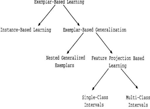
I’igure 2.1 presents a hierarchical classification of exemplar-based learning models. Instance-Based Learning (IBL) and Exemplar-Based Generalization

CHAPTER 2. SUPERVISED INDUCTIVE LEARNING MODELS

Exenplar-Based Learning

Instance-Based Learning Exemplar-Based Generalization

Nested Generalized Feature Projection Based

Exemplars Learning

Single-Class Intervals

Multi-Class Intervals

Figure 2.1. Classification of Exemplar-Based Learning models.

are two types of exemplar-based Learning. For example, instance-based learn­ ing methods [5] retain examples in memory as points, and never changes them. On the other hand, exemplar-based generalization methods make certain gener­ alizations on the training instances. One category of the exemplar-based gener­ alization is the Nested-Generalized Exemplars (NGE) model [62]. This model changes the point storage model of the instance-based learning and retains examples in the memory as axis-parallel hyperrectangles. Feature Projection Based (FPB) learning models are the basis for this thesis and can be classi­ fied as exemplar-based generalization methods. The FPB algorithms learn the concept descriptions by generalizing the projections of the training examples separately on each feature. In this thesis, we will study several supendsed inductive learning methods that can be also categorized as feature projection based algorithms. In the following sections, we will describe the IBL and NGE methods briefly. Previously developed FPB methods will be discussed in detail in Chapter 3.

2.1.1

In sta n ce-B a sed Learning

Iiislancc-Based Learning (IBL) methods extend the classical nearest neighbor algorithm, which has large storage requirements [5, 9]. IBL algorithms generate classification predictions using only specific instances. .Aha calls them also as

lazy /farnfni/algorithms since the concept description is a set of stored instances

[76]. All instances are represented as points on the (/-dimensional Euclidean space, where cl is the number of features. The concept descriptions can change incrementally after each training instance is processed. IBL algorithms do not construct extensional concept descriptions. Instead, concept descriptions are determined by how the IBL algorithm’s selected similarity and classification functions use the current set of saved instances. There are three components in the framework which describe all IBL algorithms as defined by Aha and Kibler

CHAPTER 2. SUPERVISED ISDUCTIVE LEARNING MODELS 9

1. The similarity function computes the similarity between two instances (similarities are real-valued).

2. The classification function receives the output of the similarity function and the classification performance records of the instances in the concept description, and yields a classification for instances.

■]. The concept description updater maintains records on classification per­

formance and decides which instance are to be included in the concept description.

These similarity and classification functions determine how the set of in­ stances in the concept description are used for prediction. So, IBL concept descriptions contain not only a set of instances, but also these two functions.

Several IBL algorithms have been developed: IBl. IB2. IB3, IB4 and IB5 [3. ')]. IBJ is the simplest one and it uses the similarity function computed as

CHAPTKR 2. SUPERVISED INDUCTIVE LEARNING MODELS 10 ,'<imilarity{x,y) — — di f f i f , 2:, y) = /=1 (2.1) i f / i s linear 0 if / is symbolic and xj = yj (2.2) 1 if / is symbolic and xj ^ y/

where ,r and y are the instances.

IBl is identical to the nearest neighbor algorithm except that it processes training instances incrementally and simply ignores instances with missing fea­ ture value(s). Since IBl stores all the training instances, its storage requirement is quite large. IB2 is an extension of IBl, it saves only misclassified instances reducing storage requirement. On the other hand, its classification accuracy decreases in the presence of noisy instances. IB3 aims to cope with noisy in­ stances. IB3 employs a significance test to determine which instances are good classifiers and which ones are believed to be noisy. Once an example is deter­ mined to be noisy, it is removed from the description set. IB2 and IB3 are also incremental algorithms. IBl, IB2, and IB3 algorithms assume that all features have equal relevance for describing concepts.

To study the effect of relevances of features in IBL algorithms, IB4 has been proposed by .Aha [3]. In this study, dilferent feature weights are learned for different concepts; a feature may be highly relevant to one concept and com­ pletely irrelevant to another. So, IB4 has been developed as an extension of IB3 that learns a separate set of feature weights for each concept. Weights are adjusted using a simple feedback algorithm to reflect the relative relevances of the features to describe instances. These weights are then used in IB4's similarity function which is a Euclidean weighted-distance measure of the sim­ ilarity of two instances. Multiple sets of weights are used because similarity is concept-dependent, the similarity of two instances varies depending on the target concept. IB4 decrea.ses the effect of irrelevant features on classification decisions. Therefore, it is quite successful in the presence of irrelevant features.

CHAPTER 2. SUPERVISED INDUCTIVE LEARNING MODELS 11

The problem of novelty is defined as the problem of learning when novel features are used to help describe instances. IB4. similar to its predecessors, assumes that all the features used to describe training instances are known before training begins. However, in several learning tasks, the set of describing features is not known beforehand. IB5 [3], is an e.xtension of IB4 that tolerates the introduction of novel features during training. To simulate this capability during training, IB4 simply assumes that the values for the (as yet) unused feature are missing. During training. IB4 fixes the expected relevance of the feature for classifying instances. IB5 instead updates the weight of a feature only when its value is known for both of the instances involved in a classification attem pt. IB5 can therefore learn the relevance of novel features more quickly than IB4.

Also noise-tolerant versions of instance-based algorithms have been devel­ oped by .Aha and Kibler [4]. These learning algorithms are based on a form of significance testing, that identifies and eliminates noisy concept descriptions.

2.1.2

N ested -G en era lized E xem p lars

Nested-generalized exemplar (NGE) theory is a variation of exemplar-based learning [62]. In NGE, an e.xemplar is a single training example, and a general­ ized exemplar is an axis-parallel hyperrectangle that may cover several training examples. These hyperrectangles may overlap or nest. Hyperrectangles are grown during training in an incremental manner.

Salzberg implemented NGE in a program called EACH (Exemplar-Aided Constructor of Hyperrectangles) [63]. In EACH, the learner compares new examples to those it has seen before and finds the most similar generalized e.xemplar in memory.

NGE theory makes several significant modifications to the e.xemplar-based model. It retains the notion that examples should be stored verbatim in mem­ ory. but once it stores them, it allows examples to be generalized. In NGE theory, generalizations take the form of hyperrectangles in d-dimensional Eu­ clidean space, where the space is defined by the feature values measured for

CHAPTER 2. SUPERVISED ISDUCTIVE LEARNIXG MODELS 12

each example. The hyperrectangles may be nested one inside another to arbi­ trary depth, and inner rectangles serve as exceptions to surrounding rectangles [62]. Each new training example is first classified according to the existing set of classified hyperrectangles by computing the distance from the example to each hyperrectangle. If the training example falls into the nearest hyper­ rectangle, then the nearest hyperrectangle is extended to include the training example. Otherwise, the second nearest hyperrectangle is tried. This is called as second match heuristic. If the training example falls into neither the first nor the second nearest hyperrectangle, then it is stored as a new (trivial point) hyperrectangle.

A new example will be classified according to the class of the nearest hy­ perrectangle. Distances are computed as follows: If an example does not fall into any e.xisting hyperrectangle, a weighted Euclidean distance is computed. If the example falls into a hyperrectangle, its distance to that hyperrectangle is zero. If there are several hyperrectangles having equal distances, the smallest of these is chosen. The EACH algorithm computes the distance between a new data point e and a hyperrectangle H, by measuring the Euclidean distance between these two objects as follows:

De.H = li'// where d { e , H J ) = I ^ maxf — mirif Hj uppfT ej ï> Hf_uppeT ,lower f.lower 0 otherwi se (2.3) (2.4)

where wh is the weight of the exemplar /f, wj is the weight of the feature / , e/

is the value of the / th feature on example e, Hj^^pper or Hj^ower are the upper end of the range and lower end, respectively, on / t h feature on exemplar //.

tnaxf and minj are the minimum and maximum values of that feature, and n

is the number of features recognizable on e.

The EACH algorithm finds the distance from e to the nearest face of H .

CHAPTER 2. SUPERVISED INDUCTIVE LEARNING MODELS i;{

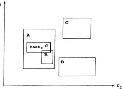
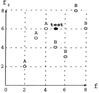
Figure 2.2. An example concept description of the EACH algorithm in a do­ main with two features.

the hyperrectangle H is a point hyperrectangle, representing an individual example, then the upper and lower values becomes ecjual.

If a training instance e and generalized e.xemplar H are of the same class, that is, a correct prediction has been made, the exemplar is generalized to in­ clude the new instance if it is not already contained in the exemplar. However, if the closest hyperrectangle has a different class then the algorithm modifies the weights of features so that the weights of the features that caused the wrong prediction is decrea.sed. This is how the E.\CH algorithm learns feature weights.

The original NGE was designed for domains with continuous features only. Discrete features require a modification of the distance and area computations for NGE.

In Figure 2.2, an example concept description constructed by the EACH algorithm is presented for a domain with two features /i and / 2. Here, there are three classes. A, B and 6’, and their descriptions are rectangles (exemplars) as shown in Figure 2.2. The rectangle A contains two smaller rectangles. B and C’, in its region. Therefore, B and C are exceptions inside the rectangle A. The NGE model allows exceptions to be stored quite easily inside hyperrectangles, and exceptions can be nested any number of levels. The test instance, that is

CHAPTER 2. SUPERVISED ISDUCTIVE LEARMNG MODELS 14

marked as test in Figure 2.2. falls into the rectangle C. since it is smaller, .so the prediction will be the class value C for this test instance.

2.1.3 F eature P r o je c tio n B ased Learning

The Feature Projection Based Learning algorithms all generalize the feature projections of the training instances in learning the concept descriptions. The pre\'iously studied techniques categorized as feature projection based learning methods under exemplar-based generalization are the Classification by Feature Partitioning (CFP) [31, 32. 71], the Classification by Overlapping Feature In­ tervals (COFI) [73], Feature Intervals .-\lgorithms (FIL) [7]. and the k Nearest .Neighbor on Feature Projections (^--NNFP) [8] algorithms. The FPB mod­ els are further classified as Single-Class Intervals and Multi-Class Intervals as shown in Figure 2.1. The CFP and the FIL algorithms are Single-Class In­ tervals algorithms. The COFI algorithm is a Multi-Class Intervals algorithm. On the other hand, the ¿-NNFP algorithm also based on feature projections can be categorized as both Single-Class and Multi-Class. The classification of unseen instances in the FPB models are based on a voting among the indi­ vidual predictions made by using the local information individually stored on each feature. The discussion of these algorithms are presented in Chapter 3 in detail.

2.2

T h e N ea rest N eigh b or C lassifier

One of the most common and simplest classification algorithms is the Nearest Neighbor (NN) algorithm. In the literature, nearest neighbor algorithms for learning from examples have been studied extensively [17, 18, 24]. Although other machine learning techniques such as decision trees [55] have been the subject of much recent experimental work, the nearest neighbor algorithms continues to stay as an accurate learning technique [64]. The nearest neighbor learning algorithms have been shown to work as well as other machine learning methods despite their simplicity [16, 18, 68]. It seems that nearest neighbor

CHAPTER 2. SUPERVISED ISDVCTIVE LEARNISG MODELS 15

met hods will continue to be cited as a basis of comparison with other methods. The NN classification algorithm is based on the assumption that examples which are closer in the instance space are of the same class. That is, unclassified ones should belong to the same class as their nearest neighbor in the training dataset. .After all the training set is stored in memory, a new example is clas­ sified as the class of the nearest neighbor among all stored training instances. Although several distance metrics have been proposed for NN algorithms [64], the most common one is the Euclidean distance metric. The Euclidean distance between two instances .r = < a’l, ,r2, ..., .r¿, Cx > and y = < Vi, ■■■yd^Cy > on

an d dimensional space is computed as:

dist{.r,y) =

1

Here wj denotes the weight for feature / and for all features tc/ = 1 in standard NN and d i f f { f , x , y ) denotes the difference between the values of instances x, and y on feature / . Note that this metric recjuires the normalization of all feature values into a same range by computing the maximum and minimum.

Although several techniques have been developed for handling unknown (missing) feature values [57, 58], the most common approach is to set them to the mean of the values on corresponding feature.

Stanfill and Waltz introduced the Value Difference Metric (VDM) to define the similarity for discrete (nominal) features and empirically demonstrated its benefits [68]. The VDM computes a distance for each pair of the different values a nominal feature can assume. It essentially compares the relative frequencies of each pair of distinct values across all classes. Two feature values have a small distance if their relative frequencies are approximately equal for all output classes. Cost and Salzberg presented a nearest neighbor algorithm that uses a

rHAPTEIi 2. SUPERVISED INDUCTIVE LEARNING MODELS H)

inodificatioii of VDM. called MVDM (Modified Value DilFerence Metric) [16]. The main difference between MVDM and VDM is that their method’s feature value differences are symmetric. This is not the case for V^DM. A comparison of MVDM and Bayesian classifier is presented in [.59].

NN algorithm can be quite effective when the features of the domain are ec|ua.lly important. However, it can be less effective when many of the features are misleading or irrelevant to classification. To avoid this problem, weakly rel­ evant features should have lower weights and strongly relevant features should have higher weights in Equation 2.5 where the weight of a feature / is rep­ resented by Wf. .Assigning different weights to the features of the instances before applying the NN algorithm distorts the feature space, modifying the importance of each feature to reflect its relevance to classification. In this way, similarity with respect to relevant features becomes more critical than similar­ ity with respect to irrelevant features. .A weight learning method for the NN algorithm will be described in Chapter 6.

In fact NN is a specialization of a more general algorithm called the k- Nearest Neighbor algorithm (A:-NN), which classifies a new instance by a ma­ jority voting among its ^ (> 1) nearest neighbors using some distance metrics in order to reduce the effect of noisy training instances.

An average-case analysis of A:-NN classifiers for Boolean threshold functions on domains with noise-free Boolean features and a uniform instance distance distribution is given by Okamoto and Satoh [53]. They observed that the performance of the ^’-NN classifier improves as k increases, then reaches a ma.ximum before starting to deteriorate, and the optimum value of k increases gradually as the number of training instances increases.

2.3

D ecision Trees

One of the most well known and widely experimented inductive learning ap­ proaches is decision trees. The original idea goes back to the work by Hunt, .Marin and Stone [37]. Other researchers have arrived independently at similar

C 7 /.4 P T E R 2. SUPERVISED INDUCTIVE LEARNING MODELS 17

metliods such as the CART system [13]. This same idea also produces ID3 [o5], PLSl [()0j, ASSISTANT [14]. The principal name for Quinlan’s famous (h'cision tree induction program is C l.-5 [58]. which is the descendant of an earlier version called ID3.

Given a set of preclassified instances, decision tree learning systems generate a tree structure that can be used to classify new instances. Each instance is described by a set of feature values, which can have either continuous (linear) or discrete (nominal) values, with the corresponding class (category) label. A dc'cision tree is either

• a leaf, indicating a class, or

• a decision node that specifies some test to be carried out on a single feature value, with one branch and subtree for each possible outcome of the test.

,A new test instance is classified by starting at the root of the tree and moving through it until a leaf is encountered. .At each nonleaf decision node, the test at the node shifts the search to the branch determined by the corresponding feature value of the test instance. When this process finally reaches a leaf node, the class label stored at the leaf node is returned as the predicted class value of the test instance.

Decision trees are built using a divide and conquer approach. The skeleton of decision tree construction from a set I' of training instances is simple. Let the classes be denoted Ci, C2, . . . , Ck- There are three possibilities:

• T contains one or more instances, all belonging to a single class Cj: The decision tree for T is a leaf identifying class Cj. •

• T contains no cases:

The decision tree is again a leaf, but the class to be associated with the leaf must be determined from information other than T. For example, C4.5 uses the most frequent class at the parent of this node.

CUAPTER 2. SUPERVISED INDUCTIVE LEARNING MODELS 18

• 7’ contains cases that belong to a mixture of classes:

In this situation, the idea is to refine T into subsets of instances that seem

to be single-class collections of instances. fesf is chosen, based on a

single feature, that has one or more mutually exclusive outcomes Oi. O2.

. . . , 0„. T is partitioned into subsets Ti, T2...T«, where T, contains

all the cases in T that have outcome (9, of the chosen test. The decision tree for T consists of a decision node identified by test, and one branch for each possible outcome. The same procedure is applied recursively for each subset of training instances produced by this test. That is, the branch leads to the decision tree constructed from the subset T,.

Each internal node contains a test that will partition the training instances. The most important decision criteria in decision tree induction is how to decide the best test on a given node. One must use some heuristics to find the best decision nodes because the problem of finding the best decision tree is NP- complete. C4.5 uses information-gain criterion to evaluate the goodness of a test. Given a set of training instances T and a test A' with n outcomes, the information can be found as the weighted sum over the subsets:

(■2.7) The information gain that is gained by partitioning T according to this test is:

gain{X) = info{T) — i nfo x{ T) (2-S) The information-gain criterion selects the test to maximize this information gain. Although this criterion gave quite good results, it has a strong bias for tests with many outcomes. To overcome this bias problem, another criterion, called gain ratio criterion is introduced [58]:

gain ratio{X) = gain{X) / split info{X)

where split info{X) is defined as:

split info{X) = - ¿ ^ X ^og2{ \ ^ )

(2.9)

(2.10)

s p l i t i n f o represents the potential information generated by dividing T into n

rUAPTER 2. SUPERVISED INDUCTIVE LEARNING MODELS 19

arising from the division. Then, the gain ratio is the proportion of information generated by the division that appears helpful.

There are three tests considered in C4.5:

• The standard test on a discrete feature, with one outcome and branch for each possible value of that feature.

• A more complex test, based on a discrete feature, in which the possible values are allocated to a variable number of groups with one outcome for each group rather than each value. This form of test is optionally invoked in C4.5.

• For a continuous feature / . a binary test with outcomes f < V and /■ > Vk based on comparing the value for / against a threshold value V. To find a threshold value, the instances are first sorted with respect to

the values of the feature / . Let those sorted values be ui, V2, . . . , Vm-

The midpoint between each n,· and is considered as a representative

threshold and rn — 1 such midpoints are all examined as a candidate threshold.

The construction process of a decision tree makes use of a hidden assump­ tion that the outcome of a test for any instance can be determined. The outcome of a test is both required when partitioning a set T into subsets T, and when classifying a test instance using a decision tree. Since every test is based on a single feature, the outcome of a test can not be determined unless the value of that feature is known. The solution of C4.5 to overcome the prob­ lem of unknown (missing) feature values in training, is to evaluate the tests by simply ignoring the instance with unknown value i.e. e.xcluding that instance in the gain calculations. Then the partition is done according to the selected test and the instance with missing value is inserted in all subsets with a probability to be in that subset. When classifying a test instance, if a decision node having a test that is unknown is reached, all possible outcomes are explored and the l)iobabilistic classifications are combined arithmetically. Then the class with the highest probability is the predicted class of the test instance.

CHAPTER 2. SUPERVISED INDUCTIVE LEARNING MODELS •20

Another problem with decision trees is that the resulting tree of C4.5 is often a very complex tree that ‘'overfits the data" b}' inferring more structure than is justified by the training instances. A decision tree is not usually simplified by deleting the whole subtree in favor of a leaf. Instead, the idea is to remove parts of the tree that do not contribute to classification accuracy on unsc'en instances, producing something less complex and thus more comprehensible. This process is known as the pruning [58].

A simpler decision tree learning approach, called IR system, is later pro­ posed by Holte [36]. It is based on the rules that classify an object on the

basis of a single feature that is, they are 1-level decision trees, called 1-rulcs

[36]. The input of the IR algorithm is a set of classified training instances and the output is a concept description in the form of 1-rule. Since each feature is considered separately in IR system, missing feature values can be simply ignored instead of ignoring the instance containing missing value. Then, one of the concept descriptions on a feature is chosen as the final concept description by selecting the one that makes the smallest error on the training dataset.

Holte used sixteen datasets, fourteen of which were selected from the collec­ tion of UCTRepository [51], to compare IR and C4.5 [36]. The main result of comparing IR and C4.5 was an insight into the tradeoff between simplicity and accuracy. IR rules are only a little less accurate (about 3 percentage points) than C4.5’s pruned decision trees on almost all of the datasets. Decision trees formed by C4.5 are considerably larger in size than 1-rules. Holte shows that simple rules such as IR are as accurate as more complex rules such as C4.5.

Another decision tree algorithm is T2 (decision trees of at most ‘2-levels) [Т2]. Its computation time is almost linear in the size of training set. The T2 algorithm is evaluated on 15 common real-world dataset. It is shown that the most of these datasets, T2 provides simple decision trees with little or no loss in accuracy compared to C4.5.

S.ADT [34] and OCT [52] are decision tree induction methods, which par­ tition instances using oblique hyperplanes. Standard decision tree techniques, such as C4.5 [58], partition a set of points with axis-parallel hyperplanes whereas oblique decision tree algorithms attempts to find hyperplanes at any

CHAPTER 2. SUPERVISED ISDVCTIVE LEAR^^l^’G MODELS 21

orientation. SADT and OCl use a randomized approach for generating de­ cision trees using non-axis-parallel hyperplanes. The purpose of these more general techniciues is to find smaller but more accurate decision trees and the ex[)eriments have shown that in some cases they produce small trees without losing predictive accuracy.

2.4

N a iv e B a y esia n C lassifier

Bayesian classifier originating from work in pattern recognition is a probabilis­ tic approach to inductive learning [24, 29]. Given the observed feature values for an instance and the prior probabilities of classes, the a posteriori probabil­ ity that an instance belongs to a class is estimated. The class with the highest estimated probability is predicted as the class of the instance. Bayesian classi­ fiers assume that features may be statistically dependent. On the other hand.

Naive Bayesian Classifier assumes that features are independent.

Bayes Decision Theory is a probabilistic approach to the problem of pattern classification. The prediction of a class label depends on probability values and it is assumed that all of the relevant probability values are known.

Suppose we are given a domain defined by d features and with k classes. The classification problem is to predict a class among k classes for the un­ seen example using the concept description induced from training instances. The probabilistic representation of a concept stores probabilistic information about each class. This information includes P{Ci), which specifies the a pri­

ori probability that one will observe a member of class C,, and a set of con­

ditional probabilities, specifying a probability distribution for each feature. From this probabilistic concept description and a given feature value vector X = < x i , ... ,aT(i > of the new example to be classified, the a posteriori prob­ ability P{Ci\x) for each cla.ss are computed. Bayes rule allows us to compute the a posteriori probability P{Ci\x) using the a priori probability P{C'i) and the class conditional density p(x|C,):

p{x\C,)P{C,) P{C,\x) =

CHAPTER 2. SUPERVISED INDUCTIVE LEARNING MODELS •22

where

P(x) = £ M x|C.)P(C’.) (2.12)

1 = 1

There are many different ways to represent classifiers. One way is in terms

of a set of discriminant functions ^¿(x). i — where k is the number of

classes. The classifier is set to assign a feature vector x to class C\ if

g,{x) > <7j(x) f o r all i ^ j. (•2.13) Thus, the classifier can be viewed as a machine that computes discriminant functions and selects the class (category) whose discriminant function has the largest value.

For the general ca.se we can let ^,(x) = / ’((?,|x), so that the maximum discriminant function corresponds to the maximum a posteriori probability. The classifier would simply select the class C, with maximum P(C ,|x).

The choice of discriminant functions is not unique. More generally, if every

gi{x) is replaced by f{gi{x))·, where / is a monotonically increasing function, the

resulting classification is unchanged. This observation can lead to significant analytical and computational simplifications. In particular, for minimum-error- rate classification, any of the following choices gives identical classification results, but some can be much simpler to understand or to compute than others [24]: ^¿(x) = P (C ,,x ) (2.14) <7.(x) = Pix\Ci)P{Q) E j . . P{x\C,)P{C,) (2.15) ^.(x) = P(x\C,)P{C,] (2.16) 5T,(x) = logP{x\Ci) + logP{Ci) (2.17)

Even though the discriminant functions can be written in a variety of forms, the decision rules are equivalent. The effect of any decision rule is to divide