Cumulant-based parametric multichannel FIR system identification methods

Cumulant-based Parametric Multichannel

FIR System IdentiJication Methodst

by M. TANKUT ~ZGEN

Middle East Technical University, Department of Electrical Engineering, Ankara, Turkey

SALEH A. ALSHEBEILI

King Saud University, Department of Electrical Engineering, Riyadh 11421, Saudi Arabia

A. ENIS GETIN

Bilkent University, Department of Electrical Engineering, Bilkent, Ankara, 06.533, Turkey

and A. N. VENETSANOPOULOS

University of Toronto, Department of Electrical Engineering, Toronto, Canada M5S IA4

ABSTRACT : In this paper, “least squares” and recursive methodsfor simultaneous idemt$ication of four nonminimum phase linear, time-invariant FIR systems are presented. The methods utilize the second- and fourth-order cumulants of outputs of the four FIR systems of which the common input is an independent, identically distributed (i.i.d.1 non-Gaussian process. The new methods can be extended to the general problem of simultaneous iden@cation of three or more FIR systems by choosing the order of the utilized cumulants to be equal to the number

of systems. To illustrate the eflectiveness of our methods, two simulation examples are

included.

I. Introduction

Nonminimum phase system (or signal) identification is an important problem

in many signal and image processing applications including data communication,

seismic signal processing and optical imaging (14).

In this paper, we address the problem of simultaneous reconstruction of the

impulse responses of four minimum or nonminimum phase FIR systems using

the power spectrum and cross-trispectrum of the output sequences. We present

parametric multichannel system identification methods.

f Portions of this paper were presented at the IEEE Signal Processing

Higher-Order Statistics, California, U.S.A., June 1993. This work is

TUBITAK, Turkey.

0 The Franklin Institute OOl&CO32/94 $7.00+0.00 @ Pergamon

Workshop on

supported by

M. Tunkut Ozgen et al.

Recent work (58) on nonminimum phase multichannel system identification

includes the work by Brooks and Nikias (5) who showed that three nonminimum

phase systems driven by an independent and identically distributed (i.i.d.) non-

Gaussian process can be reconstructed simultaneously from their output cross-

bispectrum. Their method is a nonparametric cepstral technique which computes

the complex cepstra of the impulse response sequences of the unknown systems

from the third-order cross-cumulants of output sequences. Higher order statistical

identification schemes which utilize complex cepstrum have been widely used in

practical applications (5, 9913). These schemes have some disadvantages when

poles and zeros come close to the unit circle. Our parametric methods do not suffer

from this limitation. However, they require exact knowledge of systems’ orders

and a theoretical analysis shows that they yield consistent parameter estimation

only in a class of additive colored Gaussian noise, as well as in the additive white

Gaussian noise. Experimental verification of the methods by means of simulation

examples has been provided for the case of white Gaussian noise only.

The organization of the paper is as follows. In Section II we define the problem

and introduce the basic concepts. In Section III we develop a least squares-type

method which is based on solving a system of linear equations obtained from a

relationship derived in Section II. We prove the uniqueness of the least squares

solution in Section IV by devising a recursive method to determine the unknown

impulse response parameters. We investigate the robustness of the new methods

to additive noise in Section V. In Section VI we present simulation examples,

II. Problem Definition

In this section, we describe the multichannel system identification problem.

Consider the following signal model :

vi(H) = Z;(n) + W,(n)

= i h,(k)x(n-k)+w,(n) i= 1,2,3,4 ₍₁₎

k=O

where y,(n) is the output of the ith FIR system of which the impulse response is

h,(n) ; q, is the order of the ith system; w,(n) is an additive zero-mean Gaus-

sian noise; and z!(n) is the output of the ith system in the absence of noise.

For convenience, the impulse responses, h,(n), i = 1,2,3,4, are numbered

such that q, < q2 d q3 < q4. The input sequence x(n) is assumed to be an i.i.d.

non-Gaussian process with J+(n)} = 0, E{x(n)x(n+r,)) = B*&r,),

E(x(n)x(n+s,)x(n+z2)f = /j36( rI,r2) and c.ArI,rZ,rj) = B4@rI,r2,rj) where

c,(t ,, r2, r3) denotes the fourth-order cumulants of the input x(n).

In most digital communication applications the system input, x(n), is derived

from a signal constellation which is symmetric around the origin. Therefore the

third-order cumulants of x(n) are identically zero (p, = 0). In such a case we use

the fourth-order cumulants of the system outputs. The methods developed in this

paper can be extended to the general problem of simultaneous reconstruction of

an even number of FIR systems by choosing the order of the required cumulants

FIR System Identljication Methods

to be equal to the number of systems. If the input sequence x(n) is asymmetric

around the origin, an odd number of systems can also be identified by using our

algorithm.

Let us define c, 234 (z ,, TV, z3) as the fourth-order cross-cumulant sequence of the

processes {y,(n)}~, , , i.e.

By using the fact that the fourth-order cumulants of zero-mean Gaussian noise

processes areidenticallyzero, ~,~~~(r,, z?, zj) can be related to the unknown impulse

responses (hi(n)],!=, as shown below :

The cross-trispectrum, CIZj4 (o,,w>, w3), of the output processes, {yj(n)}~= ,, is

defined as the three-dimensional Fourier transform of the cross-cumulant sequence,

~,~~~(r,,r~,r~). From (3), it follows that

C,,,,(W,,%,@,) = P4HI(OI)HZ(WZ)H3(W3)H4(_0, -wz-oJ (4)

where Hi(w) is the Fourier transform of the system impulse response hi(n).

We also need the second-order cumulant sequence, s(z) = E(z4(n)z4(n+ r)}, of

the noise free output sequence, z4(n). The power spectrum, S(o), of z4(n) is

S(w) = 82H4(W)H4(-0). (5)

2.1. A fundamental relationship

In this subsection, we derive a relationship between the second- and fourth-order

cumulants. This relationship is the basis of our multichannel system identification

method.

By multiplying both sides of Eq. (4) by H,(w, +w2+03) and using (5) we get

N,(o, +%+03)C1234 (WI,%,~X) = &H,(OI)HZ(O*)H3(0j)S(OI+W*+03)

(6)

where E = fi4/fi2. By taking the inverse Fourier transform of both sides of (6) we

obtain the following relationship :

z h4G)c1234(~1 - z,z,-i,z,-ii) =E $ h,(i)hz(~~-~,+i)hj(t3-~,+i)~(~,-i)

I= 0 i=O

(7)

which relates the impulse responses, {h,(n)},?, ,, to the second-order cumulants,

s(n), of the sequence z4(n) and the fourth-order cross-cumulants, c, 234(t ,, r2, r,),

Vol. 33lB, No. 2. pp. 145-155. 1994

M. Tankut &gen

et al.

of the output sequences,

{yi(n)},?= ,

. This relationship is the four-channel version

of an equation used in some parametric system identification techniques (11, 14).

Equation (7) is very important because it allows us to estimate the impulse

responses,

{h,(n)},~~ ,

, by solving an overdetermined system of linear equations.

III. Least Squares (LS) Solution

In this section, we develop a least squares method for reconstructing the impulse

response sequences,

(h,(n))!= ,,

from the second-order cumulants and the fourth-

order cross-cumulants by using Eq. (7). First, we assume without loss of generality

that (hi(n)},!, , is scaled such that hi(O) = 1,

i =

1,2,3,4. Then, Eq. (7) can be

arranged as follows :

c12~(r1,r2,23) = s g hl(W2(r2-r1 +i)h3(rj-7, +i)s(r, -i)

r=O

-,s, hd(i)c ,*34(2*-i,22-i,~3-i). (8)

By concatenating (8) for (r ,, TV, zj) E S where S is a region which is described below,

we obtain the following overdetermined system of linear equations :

where

d=Mr ₍₉₎

r = Ml). ..h&&sh,(l). . .Eh,(qd&(l) . . .~hz(qz)Ehdl)

. . .Eh3(q3)

~hz(qz)h~(qd~h,U)h2(l)h3(1).

. . Eh,(q,)h,(q,)h,(q,)lT

is a (q4+(qI+l)(q2+l)(q3+l)) column vector, d = [c~~~~(T~,z~,T~):

(T~,z~,T~)ES]~ is an

N(qlrq2,q3,q4)

column vector, and M is a matrix of size N(q,,q2,q3,q4)x(q4+(q,+1)(q2+l)(q,+1))ofwhichtheentriesaredetermined

according to (8).

N(q,,q,,q,,q,)

is the number of points in the region S

which is determined as follows. It follows from (3) that c, 2,4(~, , z 2, z ,) is nonzero

for

-q4 d zI < ql, -q4 d z2 dq?

and

-q4<

zj < q3.

Hence, the left hand

side of (7),

C:J,h,(.) z c,234(21-i, r,-i,

s3-i),

is nonzero for

-q4 < 2, < q,+q4,

-q4 ,< 72 < q2+q4, and -q4 d s3 G q3+q4.

In addition, we should maintain

that the

h2(r2-T,+i)h3(T3-r,+i)

term at the right hand side of (7) is nonzero,

yielding

O<z,-z,+i<q,,

O<r,--z,+i<q,

for

i=O,l,2,...,q,.

This leads

to

-ql < s2-7, ,( q2 and

-q, < z3-zI

< q3.

Thus, the region S is defined by

the following set,

S= ((Zlrt2r~3): -q4 < 71 d ql+q4, -94 d z2 d q2+q4, -q4 < 73 < q3+q4, -_41 d 72-z1 G q,,

-91 d

z3---sI <

q3).

(10)

By counting the number of points in this region, we obtain the size of the column

vector d, Nq,, q2, q3, q4), as

FIR System IdentiJication Methods

Wq,,q,,q3,q4) = 41(41+1)(2q,+~)P+(qz+q3+2)q,(q,+1)

+2(q,+l)(q,+l)(q3+1)+(2q,-q,-l)(q,+q*+l)(qI+q~+1). (11)

The least squares solution of the overdetermined system of linear equations given

by (9) is

r = (MTM)-‘MTd. (12)

h,(l), h,(2), . . . , h4(q4) can then be determined as the first q4 elements of the vector

r. The other impulse response coefficients {hi(n)},3_, can directly be obtained by

dividing the corresponding element of r by r(q, + l), which is E.

However, directly obtained results could be inaccurate due to measurement noise

and estimation errors. In that case, we identify {h,(n)},3,, by using a method (11)

that is based on the singular value decomposition (SVD). This method exploits all

the available information provided by the vector r except the information contained

in the terms .zhl(i)hZ(j)h3(k).

We form three matrices R[h,, h2], R[h,, h3], R[h,, h3] from the vector r as follows :

- 1 _h,(l) h,(2) ... _{hi (qj)}

hi(l) hi(l)hj(l) h,(l)hj(2) . .. hi(l)hj(qj)

RF,, hj] = E hi(z) h,(2)hj(l) ht(2)hj(2) . . . hz(2)h,(qj) (13)

. .

_h,(q;) hi(q . . . . . . hi(q _

where i, j = 1,2,3 and i # j. The matrix R[hi, hj] is of rank one and can be written

in the following form

R[hi, hj] = E 1 hi(l) hi(z) hi(qi)

[l h,(l) hj(2) ...

h,(q,)l.

(14)

The unknown impulse response sequences h,(n) and hi(n) can be identified from

R[hi, hj] using the singular value decomposition, i.e.

R[hi, hj] = ZVUT ₍₁₅₎

where V is a (qt+ 1) by (qj+ 1) matrix which has a special diagonal form. The

diagonal elements of V are the singular values of R[hi, hj]. The columns of the

orthogonal matrix Z, zI,z2,. . . , zqi+ ,, are the left singular vectors of Rbi, hj] and the

columns of the orthogonal matrix U, ul, u2,. . . , upi+ ,, are the right singular vectors

of R[hi, hi]. Since R[hi, hj] is of rank one, it has only one nonzero singular value of

which the corresponding singular vectors determine the impulse responses h,(n)

and h,(n). From the properties of the SVD, it can be shown that (15)

and

h,(n)=k,z,(n) O<ndq, (16)

Vol. 33lB. No. 2, pp. 145-155, 1994

M. Tankut ijzgen et al.

h,(n) = k+,(n)

0 d

n < q,

(17)

where k, and kz are constants chosen to scale the singular vectors, z, and u,, so that

h,(O) = h,(O) = 1. The above step provides two different values for each impulse

response sequence h,(n), since it is used twice in the matrices R[h,, hJ, R[h,, h3],

R[h2, h3]. The arithmetic mean of them can be taken as the final result.

We should mention that the assumption that only one singular value of R[hi, hj]

is nonzero is only theoretically valid. In practice, due to noise and estimation errors,

there may be many nonzero singular values, but only a single dominant one. In

such a case we keep the dominant singular value and its corresponding singular

vectors. Also, the term “least squares” used in this section does not imply the

optimality of the method in the sense of minimizing the mean-square estimation

error. It refers to the least squares solution of Eq. (9).

IV. Uniqueness of the LS Solution and the Recursive Method

The least squares method described in the previous section yields a unique (least

squares) solution if the matrix M has full rank. In order to show that the matrix

M is of full rank we first show that the elements of the unknown vector, r, can

uniquely be determined from (7) using a recursive algorithm. From this fact, we

will be able to derive the unicity of the least squares approach.

By setting z , = t? = 73 = -q, in (7) and by using the fact that h,(O) = 1,

i = 1,2,3,4, we obtain

E _ cl234 ( -q4r~Iq4, -q4)

SC-_q4) .

(18)

Similarly, by setting s, = -q4 only, we obtain

c1734(-q4,T2,T3) EhZ(Z2+q4P3(T3+q4) =

--~----s(_q4)

52 = -q,,.. .9q2-q4. 73 = -q,,...,q3-q,, (19) and c,,,,(-q4,T2,~3) k,(Tz+q,M,(T,+q,) = =-q4) C1234(-q4,T2rTJ)_~ c201 = G234(-q4, -q4r -q4)

We can recover h,(n) and h,(n) by setting zi = -q, and r2 = -q4 in the above

equation, i.e. and c,214(-q4, -q4,~3) h,(z,+q,) = cm;;;l(zmq m_q 47 49 _mym) T3 = -44, 4 . . . 3q2-94 rq3-q4.

(21)

(22)

Setting ri = -q4 in (7) yields 150

FIR System Ident$cation Methods

Eh,(T, +qdh2(~2+qd =

C,*34(~,,~2,

-q4)

d--94)

71 = -94,

. .

..q1-q4. and r2 = -q4,...,q2-q4 (23) c,234(zI,z2> -94)

h,(r, +qhM~2+q4) =

c,234(_q 4, _q 47 _q ,. 4

We can recover h ,(n) by setting r2 = - q4 in the above equation, as

(24)

h,(T, +q4) =

:!??&_-y4r

-q4)

c,234(-q4, _q4, _q4)

71 = -q‘b...,q1-q4.

(25)

Similarly, we set r2 = -q4 in (7) and we obtain

-94753)

Ehl(ZI +q4)h,(t~+q4) = (“i”(:(‘_y~4j~~ _{51 = -q4,...rq1-q4,}

73 = -q4,...,q3-q4. (26)

At this point, we compute h4(n), 1 < n < q4, as follows. We start with the assump-

tion that h4(0) = 1. For n = 1 to Lq4/2J, L-J denoting the greatest integer smaller

than the number, we set rl = -q4+n, z2 = q2-q4+n, and r3 = q3-q4+n in (7)

and we recursively obtain

n- I

-,;“A

I 1 c1234(-q4+n-ii,

(1

q2-q4+n-ii, q3-q4+n-i)

1

. (27)

By setting t I = q1 +q4, z2 = q4, z3 = q4 in (7)

Eh

I

(4

I

)s(qJ

h4(q4) =

p1234cq,, o, o) .

(28)

Then, for n = 1 to Lq4/2_l, we set rl = q1+q4-n, z2 = q4-n, 73 = q4-n in (7)

and we recursively obtain

hk4-n) =

c-,23;d~o~

EhI(qI)4q4-n)

2 9

I,- I

- 1 h4(q4-i)c1234(q,

i=

0

-n+i, -n+i, -n+i)

1

. (29)

We note that Lq4/2 J = q4/2 if q4 is even, and Lq4/2 J = (q4- 1)/2 if q4 is odd.

Finally, we are ready to recover the unknown parameters

{Eh,(i)h2(z2_z,+i)h,(23-~,+~)}. F or n = 0 to Lq,/2], we set r, = -q4+n in

(7) and recursively compute

Vol. 3318, No. 2, pp. 145~155, 1994

M. Tunkut Ozgen et al.

ch,(n)h,(z,+q,)h,(z3+q4) =

&

L

i

h,(i)c,,,,(-q,+n--,Z*--,Z3--) i=n n- I - 1 Eh,(i)h2(5*+q4-n+i)h,(z,+q,-n+i)s(-qqq+n-_) ) (30) i= 0 1

for z2 = -q4,. . . ,q2-q4 and z3 = -q4,. . . , q3 - q4. The above recursive formula

requires the knowledge of {h,(n)} and (shahs} to compute

{~h,(i)h2(t2-~,+i)h3(~3--,++)}. N ow,wesetr,=r,=r,=q,+q,in(7):

CA (q,)h (q )A (q_) =

h4(q4)C1234(ql,qZ,q3)

2 2 3 3

G4)

(31)

Then, we start from &,(ql)h2(q2)h3(q3) by setting t, = q, +q4-n in (7) for n = 0

to Lq ,/2 J, and we recursively compute

eh,(q, -@b(~2-q4)h3(~3-q4) = &[ j_ h4G)C,234(ql +q4-fl-->T,r-i, z3-i)

i YI n

- ; Eh,(Llh2(z2-q, -q4+n+zpz,(t,-q, -qq4+n+i)s(q,+q,-n-i) ,

r=ylm”+l

1

(32)

for z2 = q4,. . . ,q2+q4 and r3 = q,,. . .,q3+q4.

The recursive algorithm described above uses Eq. (7) only for certain values of

t ,, zZ, r3 to uniquely determine the unknown vector r. Therefore it is equivalent to

choosing linearly independent rows of the matrix M and solving the system of

linear equations formed by these independent rows. It follows then that there are

q,+(l+q,)(l +q2)(1 +q3) linearly independent rows of M where this number is

the number of unknowns in the system of linear equations given by (9). Hence the

rank of the matrix M is q4+(l +q,)(l +q2)(l +q,). Since M has full rank, there is

a unique least squares solution.

V. Robustness to Additive Gaussian Noise

In practical applications, the received signals, {~,(n))p, ,, are usually the noise

corrupted version of the system outputs,

{~,(n)},~_

,

In this section, we consider the

case where the noise terms {w,(Pz)},~=~ are Gaussian noise processes, independent

of each other and {~,(n)},~_, [see Eq. (l)].

For zero-mean Gaussian processes, cumulants of order greater than two are

identically zero. Hence the fourth-order cumulants of

{y~(n)}~=

,

are not affected

by additive Gaussian noise. However, the second-order cumulants are affected by

the presence of Gaussian noise. The methods described in previous sections use the

second-order cumulant sequence S(Z) of the noiseless case system output z4(y1),

instead of the second-order cumulant sequence sp4(z) of v,(n). They are related to

each other as follows :

FIR System Ident$cation Methods

Syq(T)

= S(T)

+sIv4(4

(33)

where sW4(r) is the second-order cumulant sequence of wq(n). In practice we can

only estimate s,,,(r), not s(z). It follows from (27))(29) and (30))(32) that the

recursive method described in Section IV uses samples of s(z) for which

q4-Lq4/2_1

d Id d

q4. If the second-order cumulants of the additive noise, sWq(r),

are nonzero for lags in the range Izl d q where q = q4- Lq4/2]- 1 the recursive

method will not be affected by the presence of noise as sYd(z) = s(r) for q < ITI < q4.

Consequently, uniqueness and consistency of the LS solution will remain unaffected

if the rows of the matrix M which contain the samples of s,,,~(z) are removed. Both

the least squares and recursive solutions are robust to additive white Gaussian

noise because s,,~(T) is nonzero only for r = 0.

VI. Simulation Examples

Consider the following set of systems

y , (n) = x(n) - 0.6x(n - 1) + w , (n)

y,(n) = x(n) +0.75x(n- 1) + w*(n)

y3(n) = x(n)+OSx(n- 1) - 1.25x(n-2)+ w,(n)

y,(n) = x(n)-0.375x(n- 1)+0.8x(n-2)+w4(n) (34)

where the input signal, x(n), is a zero mean, i.i.d. sequence with /I1 = 5, j13 = 0

and /I4 = -34. The noise terms, (w,(n)}:_ ,, are zero-mean, white Gaussian pro-

cesses with variance 1, and they are uncorrelated with each other and with the

input signal x(n).

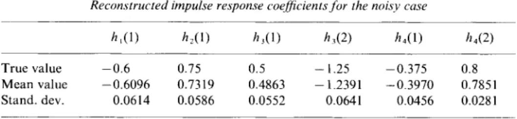
In our simulation examples the data records (N = 2048), {y;(n)},?, ,

(n = 0, 1, . ,2047), were generated by the above set of systems. The impulse

response coefficients of the unknown systems were estimated by using the LS

method for 100 output realizations for the noise-free case where noise processes,

{wj(n)}P, ,, are eliminated in the signal model, as well as the noisy case. The mean

value and the standard deviation for each impulse response coefficient were com-

puted over 100 realizations. For the noisy case, rows of the coefficient matrix M

which contain the value, sY4(0), were removed. Experimental results are presented

in Tables I and II. It is observed that the mean values are not significantly different

for the noise-free and noisy cases. However, standard deviations are slightly larger

for the noisy case.

TABLE I

Reconstructed impulse response co@icients for the noise-free case

True value Mean value Stand. dev. h,(l) h,(l) -0.6 0.75 -0.6121 0.7307 0.0422 0.0380 h,(l) h,(2) h,(l) h,(2) 0.5 -1.25 -0.375 0.8 0.4866 - 1.2340 -0.3931 0.7863 0.0366 0.0421 0.0358 0.0173 Vol. 33lB, No. 2, pp. 145-155, 1994

M. Tankut aqen et al.

TABLE II

Reconstructed impulse response coefJicients,for the noisy case

h,(l) hdI) h,(l) h,(2) ha(l) h,(2)

True value -0.6 0.75 0.5 - 1.25 -0.375 0.8

Mean value -0.6096 0.7319 0.4863 - 1.2391 -0.3970 0.7851 Stand. dev. 0.0614 0.0586 0.0552 0.0641 0.0456 0.028 1

Complex-cepstra based system identification methods produce poor results when

system zeros are close to the unit circle (5, 9, 10). Our parametric methods do not

suffer from this limitation. For example, in (34) h,(n) and h,(n) have zeros at

- I .3956, 0.8956 and 0. I875 f i0.8746, respectively. Although the last three zeros

are close to the unit circle, our LS method produced good estimates of them.

The new methods require exact knowledge of systems’ orders. In (11) an efficient

system order determination scheme was developed for single channel system identi-

fication. This scheme is based on the single channel version of our fundamental

equation (7). A reliable multichannel system order estimation scheme can be

developed as in (11).

A consistent behavior of the new methods has been observed in all the simulation

examples tried for the case of white Gaussian noise. Numerical stability of

our algorithms has not been examined in the case of colored Gaussian noise

disturbance.

VII. Conclusion

In this paper new methods for simultaneous identification of four minimum or

nonminimum phase LTT FIR systems driven by an i.i.d. non-Gaussian process are

presented. Our methods, a least squares (LS) method and a recursive method, are

parametric and use the second- and fourth-order cumulants of the system outputs

in an appropriate domain of support. The recursive method is developed to prove

the uniqueness of the least squares solution. The new methods can be extended to

the more general problem of simultaneous identification of three or more systems

by using second-order cumulants and system output cumulants of order being

equal to the number of systems to be identified. We experimentally observed that

the LS method yields consistent parameter estimation in the case of white Gaussian

noise.

Acknowledgement

We thank the anonymous reviewer for his careful review and helpful comments.

References

(1) L. Chapparo and L. Luo, “Identification of two-dimensional systems using sum-of-

cumulants”, “Proc. 1992 International Conf. on Acoustics, Speech, and Signal

Processing (ICASSP’92)“, pp. V-481-484, IEEE Press, 1992.

FIR System Ident$cation Methods (2) A. T. Erdem, “A nonredundant set for the bispectrum of 2-D signals”, “Proc. 1993

Int. Conf. on Acoustics , Speech, and Signal Processing (ICASSP’93)“, pp. IV- I88 191, IEEE Press, 1993.

(3) J. M. Mendel, “Tutorial on higher-order statistics (spectra) in signal processing and system theory : theoretical results and some applications”, IEEE Proc., Vol. 79, pp.

278305, 199 I.

(4) C. L. Nikias and M. R. Raghuveer, “Bispectrum estimation : a digital signal processing framework”, IEEE Proc., Vol. 75, pp. 869-891, 1987.

(5) D. H. Brooks and C. L. Nikias, “The cross-bicepstrum : properties and applications for signal reconstruction and system identification”, in “Proc. ICASSP-9 I “, Toronto, pp. 3433-3436, May 1991.

(6) P. Comon, “MA identification using fourth order cumulants”, Signal Processing, Vol. 26, pp. 381-388, 1992.

(7) G. B. Giannakis, Y. Inouye and J. M. Mendel, “Cumulant based identification of multichannel MA models”, IEEE Trans. Automat. Control, Vol. 34, No. 7, pp. 7833 787, 1989.

(8) A. Swami, G. B. Giannakis and S. Shamsunder, “A unified approach to modeling multichannel ARMA processes using cumulants”, IEEE Trans. Signal Processing,

in press.

(9) S. Alshebeili and A. E. Cetin, “A phase reconstruction algorithm from bispectrum”,

IEEE Trans. Geosci. Remote Sensing, Vol. 28, pp. 166171, March 1990.

(10) S. A. Alshebeili, A. E. Cetin and A. N. Venetsanopoulos, “Identification of non- minimum phase MA systems using cepstral operations on slices of higher order spectra”, IEEE Trans. Circuits Systems : Purt II Analogy Digitul Signal Processing,

Vol. 39, pp. 634637, 1992.

(11) S. A. Alshebeili, A. N. Venetsanopoulos and A. E. Cetin, “Cumulant based identi- fication approaches for nonminimum phase FIR systems”, IEEE Trans. Signal Processing, Vol. 41, No. 4, pp. 15761588, 1993.

(12) A. E. Cetin, “An iterative algorithm for signal reconstruction from bispectrum”, IEEE Trans. Signal Processing, Vol. 39, pp. 2621-2629, 1991.

(13) R.L. Pan and C. L. Nikias, “The complex cepstrum of higher order cumulants and nonminimum phase system identification”, IEEE Trans. Signal Processing, Vol. 38,

pp. 186205, 1988.

(14) J. K. Tugnait, “Approaches to FIR system identification with noisy data using higher order statistics”, IEEE Trans. Acoust. Speech Signal Processing, Vol. 38, pp. 1307-

1317, 1990.

(15) G. H. Golob and C. F. Van Loan, “Matrix Computations”, The Johns Hopkins University Press, 1983.

Received : 4 August 1993 Accepted : 26 October 1993

Vol. 33lB, No. 2, pp. 145-155, 1994