published as:
Confirmation of a charged charmoniumlike state
Z_{c}(3885)^{∓} in e^{+}e^{-}→π^{±}(DD[over
¯]^{*})^{∓} with double D tag
M. Ablikim et al. (BESIII Collaboration)
Phys. Rev. D 92, 092006 — Published 9 November 2015
DOI:
10.1103/PhysRevD.92.092006
with double D tag
M. Ablikim1, M. N. Achasov9,f, X. C. Ai1, O. Albayrak5, M. Albrecht4, D. J. Ambrose44, A. Amoroso49A,49C, F. F. An1,
Q. An46,a, J. Z. Bai1, R. Baldini Ferroli20A, Y. Ban31, D. W. Bennett19, J. V. Bennett5, M. Bertani20A, D. Bettoni21A,
J. M. Bian43, F. Bianchi49A,49C, E. Boger23,d, I. Boyko23, R. A. Briere5, H. Cai51, X. Cai1,a, O. Cakir40A,b, A. Calcaterra20A, G. F. Cao1, S. A. Cetin40B, J. F. Chang1,a, G. Chelkov23,d,e, G. Chen1, H. S. Chen1, H. Y. Chen2, J. C. Chen1,
M. L. Chen1,a, S. Chen Chen41, S. J. Chen29, X. Chen1,a, X. R. Chen26, Y. B. Chen1,a, H. P. Cheng17, X. K. Chu31, G. Cibinetto21A, H. L. Dai1,a, J. P. Dai34, A. Dbeyssi14, D. Dedovich23, Z. Y. Deng1, A. Denig22, I. Denysenko23, M. Destefanis49A,49C, F. De Mori49A,49C, Y. Ding27, C. Dong30, J. Dong1,a, L. Y. Dong1, M. Y. Dong1,a, S. X. Du53,
P. F. Duan1, J. Z. Fan39, J. Fang1,a, S. S. Fang1, X. Fang46,a, Y. Fang1, L. Fava49B,49C, F. Feldbauer22, G. Felici20A,
C. Q. Feng46,a, E. Fioravanti21A, M. Fritsch14,22, C. D. Fu1, Q. Gao1, X. L. Gao46,a, X. Y. Gao2, Y. Gao39, Z. Gao46,a, I. Garzia21A, K. Goetzen10, W. X. Gong1,a, W. Gradl22, M. Greco49A,49C, M. H. Gu1,a, Y. T. Gu12, Y. H. Guan1,
A. Q. Guo1, L. B. Guo28, R. P. Guo1, Y. Guo1, Y. P. Guo22, Z. Haddadi25, A. Hafner22, S. Han51, X. Q. Hao15,
F. A. Harris42, K. L. He1, X. Q. He45, T. Held4, Y. K. Heng1,a, Z. L. Hou1, C. Hu28, H. M. Hu1, J. F. Hu49A,49C, T. Hu1,a, Y. Hu1, G. M. Huang6, G. S. Huang46,a, J. S. Huang15, X. T. Huang33, Y. Huang29, T. Hussain48, Q. Ji1, Q. P. Ji30,
X. B. Ji1, X. L. Ji1,a, L. W. Jiang51, X. S. Jiang1,a, X. Y. Jiang30, J. B. Jiao33, Z. Jiao17, D. P. Jin1,a, S. Jin1,
T. Johansson50, A. Julin43, N. Kalantar-Nayestanaki25, X. L. Kang1, X. S. Kang30, M. Kavatsyuk25, B. C. Ke5, P. Kiese22, R. Kliemt14, B. Kloss22, O. B. Kolcu40B,i, B. Kopf4, M. Kornicer42, W. Kuehn24, A. Kupsc50, J. S. Lange24, M. Lara19, P. Larin14, C. Leng49C, C. Li50, Cheng Li46,a, D. M. Li53, F. Li1,a, F. Y. Li31, G. Li1, H. B. Li1, H. J. Li1, J. C. Li1, Jin Li32,
K. Li13, K. Li33, Lei Li3, P. R. Li41, T. Li33, W. D. Li1, W. G. Li1, X. L. Li33, X. M. Li12, X. N. Li1,a, X. Q. Li30, Z. B. Li38,
H. Liang46,a, J. J. Liang12, Y. F. Liang36, Y. T. Liang24, G. R. Liao11, D. X. Lin14, B. J. Liu1, C. X. Liu1, D. Liu46,a, F. H. Liu35, Fang Liu1, Feng Liu6, H. B. Liu12, H. H. Liu16, H. H. Liu1, H. M. Liu1, J. Liu1, J. B. Liu46,a, J. P. Liu51,
J. Y. Liu1, K. Liu39, K. Y. Liu27, L. D. Liu31, P. L. Liu1,a, Q. Liu41, S. B. Liu46,a, X. Liu26, Y. B. Liu30, Z. A. Liu1,a,
Zhiqing Liu22, H. Loehner25, X. C. Lou1,a,h, H. J. Lu17, J. G. Lu1,a, Y. Lu1, Y. P. Lu1,a, C. L. Luo28, M. X. Luo52, T. Luo42, X. L. Luo1,a, X. R. Lyu41, F. C. Ma27, H. L. Ma1, L. L. Ma33, M. M. Ma1, Q. M. Ma1, T. Ma1, X. N. Ma30, X. Y. Ma1,a,
F. E. Maas14, M. Maggiora49A,49C, Y. J. Mao31, Z. P. Mao1, S. Marcello49A,49C, J. G. Messchendorp25, J. Min1,a,
R. E. Mitchell19, X. H. Mo1,a, Y. J. Mo6, C. Morales Morales14, K. Moriya19, N. Yu. Muchnoi9,f, H. Muramatsu43, Y. Nefedov23, F. Nerling14, I. B. Nikolaev9,f, Z. Ning1,a, S. Nisar8, S. L. Niu1,a, X. Y. Niu1, S. L. Olsen32, Q. Ouyang1,a,
S. Pacetti20B, Y. Pan46,a, P. Patteri20A, M. Pelizaeus4, H. P. Peng46,a, K. Peters10, J. Pettersson50, J. L. Ping28, R. G. Ping1,
R. Poling43, V. Prasad1, M. Qi29, S. Qian1,a, C. F. Qiao41, L. Q. Qin33, N. Qin51, X. S. Qin1, Z. H. Qin1,a, J. F. Qiu1, K. H. Rashid48, C. F. Redmer22, M. Ripka22, G. Rong1, Ch. Rosner14, X. D. Ruan12, V. Santoro21A, A. Sarantsev23,g,
M. Savri´e21B, K. Schoenning50, S. Schumann22, W. Shan31, M. Shao46,a, C. P. Shen2, P. X. Shen30, X. Y. Shen1,
H. Y. Sheng1, M. Shi1, W. M. Song1, X. Y. Song1, S. Sosio49A,49C, S. Spataro49A,49C, G. X. Sun1, J. F. Sun15, S. S. Sun1,
X. H. Sun1, Y. J. Sun46,a, Y. Z. Sun1, Z. J. Sun1,a, Z. T. Sun19, C. J. Tang36, X. Tang1, I. Tapan40C, E. H. Thorndike44, M. Tiemens25, M. Ullrich24, I. Uman40B, G. S. Varner42, B. Wang30, D. Wang31, D. Y. Wang31, K. Wang1,a, L. L. Wang1,
L. S. Wang1, M. Wang33, P. Wang1, P. L. Wang1, S. G. Wang31, W. Wang1,a, W. P. Wang46,a, X. F. Wang39, Y. D. Wang14,
Y. F. Wang1,a, Y. Q. Wang22, Z. Wang1,a, Z. G. Wang1,a, Z. H. Wang46,a, Z. Y. Wang1, Z. Y. Wang1, T. Weber22, D. H. Wei11, J. B. Wei31, P. Weidenkaff22, S. P. Wen1, U. Wiedner4, M. Wolke50, L. H. Wu1, L. J. Wu1, Z. Wu1,a, L. Xia46,a,
L. G. Xia39, Y. Xia18, D. Xiao1, H. Xiao47, Z. J. Xiao28, Y. G. Xie1,a, Q. L. Xiu1,a, G. F. Xu1, J. J. Xu1, L. Xu1, Q. J. Xu13,
X. P. Xu37, L. Yan49A,49C, W. B. Yan46,a, W. C. Yan46,a, Y. H. Yan18, H. J. Yang34, H. X. Yang1, L. Yang51, Y. Yang6, Y. X. Yang11, M. Ye1,a, M. H. Ye7, J. H. Yin1, B. X. Yu1,a, C. X. Yu30, J. S. Yu26, C. Z. Yuan1, W. L. Yuan29, Y. Yuan1,
A. Yuncu40B,c, A. A. Zafar48, A. Zallo20A, Y. Zeng18, Z. Zeng46,a, B. X. Zhang1, B. Y. Zhang1,a, C. Zhang29, C. C. Zhang1,
D. H. Zhang1, H. H. Zhang38, H. Y. Zhang1,a, J. Zhang1, J. J. Zhang1, J. L. Zhang1, J. Q. Zhang1, J. W. Zhang1,a,
J. Y. Zhang1, J. Z. Zhang1, K. Zhang1, L. Zhang1, X. Y. Zhang33, Y. Zhang1, Y. N. Zhang41, Y. H. Zhang1,a, Y. T. Zhang46,a, Yu Zhang41, Z. H. Zhang6, Z. P. Zhang46, Z. Y. Zhang51, G. Zhao1, J. W. Zhao1,a, J. Y. Zhao1,
J. Z. Zhao1,a, Lei Zhao46,a, Ling Zhao1, M. G. Zhao30, Q. Zhao1, Q. W. Zhao1, S. J. Zhao53, T. C. Zhao1, Y. B. Zhao1,a, Z. G. Zhao46,a, A. Zhemchugov23,d, B. Zheng47, J. P. Zheng1,a, W. J. Zheng33, Y. H. Zheng41, B. Zhong28, L. Zhou1,a,
X. Zhou51, X. K. Zhou46,a, X. R. Zhou46,a, X. Y. Zhou1, K. Zhu1, K. J. Zhu1,a, S. Zhu1, S. H. Zhu45, X. L. Zhu39,
Y. C. Zhu46,a, Y. S. Zhu1, Z. A. Zhu1, J. Zhuang1,a, L. Zotti49A,49C, B. S. Zou1, J. H. Zou1
(BESIII Collaboration)
1 Institute of High Energy Physics, Beijing 100049, People’s Republic of China 2 Beihang University, Beijing 100191, People’s Republic of China
3 Beijing Institute of Petrochemical Technology, Beijing 102617, People’s Republic of China 4 Bochum Ruhr-University, D-44780 Bochum, Germany
5 Carnegie Mellon University, Pittsburgh, Pennsylvania 15213, USA 6 Central China Normal University, Wuhan 430079, People’s Republic of China
7 China Center of Advanced Science and Technology, Beijing 100190, People’s Republic of China
8 COMSATS Institute of Information Technology, Lahore, Defence Road, Off Raiwind Road, 54000 Lahore, Pakistan 9 G.I. Budker Institute of Nuclear Physics SB RAS (BINP), Novosibirsk 630090, Russia
10GSI Helmholtzcentre for Heavy Ion Research GmbH, D-64291 Darmstadt, Germany 11 Guangxi Normal University, Guilin 541004, People’s Republic of China
12 GuangXi University, Nanning 530004, People’s Republic of China 13 Hangzhou Normal University, Hangzhou 310036, People’s Republic of China 14 Helmholtz Institute Mainz, Johann-Joachim-Becher-Weg 45, D-55099 Mainz, Germany
15 Henan Normal University, Xinxiang 453007, People’s Republic of China
16 Henan University of Science and Technology, Luoyang 471003, People’s Republic of China 17Huangshan College, Huangshan 245000, People’s Republic of China
18Hunan University, Changsha 410082, People’s Republic of China 19 Indiana University, Bloomington, Indiana 47405, USA
20(A)INFN Laboratori Nazionali di Frascati, I-00044, Frascati, Italy; (B)INFN and University of Perugia, I-06100, Perugia,
Italy
21 (A)INFN Sezione di Ferrara, I-44122, Ferrara, Italy; (B)University of Ferrara, I-44122, Ferrara, Italy 22Johannes Gutenberg University of Mainz, Johann-Joachim-Becher-Weg 45, D-55099 Mainz, Germany
23 Joint Institute for Nuclear Research, 141980 Dubna, Moscow region, Russia
24 Justus Liebig University Giessen, II. Physikalisches Institut, Heinrich-Buff-Ring 16, D-35392 Giessen, Germany 25 KVI-CART, University of Groningen, NL-9747 AA Groningen, The Netherlands
26Lanzhou University, Lanzhou 730000, People’s Republic of China 27Liaoning University, Shenyang 110036, People’s Republic of China 28 Nanjing Normal University, Nanjing 210023, People’s Republic of China
29 Nanjing University, Nanjing 210093, People’s Republic of China 30Nankai University, Tianjin 300071, People’s Republic of China
31 Peking University, Beijing 100871, People’s Republic of China 32Seoul National University, Seoul, 151-747 Korea 33Shandong University, Jinan 250100, People’s Republic of China 34Shanghai Jiao Tong University, Shanghai 200240, People’s Republic of China
35 Shanxi University, Taiyuan 030006, People’s Republic of China 36 Sichuan University, Chengdu 610064, People’s Republic of China
37 Soochow University, Suzhou 215006, People’s Republic of China 38Sun Yat-Sen University, Guangzhou 510275, People’s Republic of China
39Tsinghua University, Beijing 100084, People’s Republic of China
40 (A)Istanbul Aydin University, 34295 Sefakoy, Istanbul, Turkey; (B)Dogus University, 34722 Istanbul, Turkey; (C)Uludag
University, 16059 Bursa, Turkey; (D)Near East University, Nicosia, North Cyprus, 10, Mersin, Turkey
41 University of Chinese Academy of Sciences, Beijing 100049, People’s Republic of China 42 University of Hawaii, Honolulu, Hawaii 96822, USA
43 University of Minnesota, Minneapolis, Minnesota 55455, USA 44University of Rochester, Rochester, New York 14627, USA
45 University of Science and Technology Liaoning, Anshan 114051, People’s Republic of China 46 University of Science and Technology of China, Hefei 230026, People’s Republic of China
47 University of South China, Hengyang 421001, People’s Republic of China 48 University of the Punjab, Lahore-54590, Pakistan
49 (A)University of Turin, I-10125, Turin, Italy; (B)University of Eastern Piedmont, I-15121, Alessandria, Italy; (C)INFN,
I-10125, Turin, Italy
50 Uppsala University, Box 516, SE-75120 Uppsala, Sweden 51Wuhan University, Wuhan 430072, People’s Republic of China 52Zhejiang University, Hangzhou 310027, People’s Republic of China 53Zhengzhou University, Zhengzhou 450001, People’s Republic of China a
Also at State Key Laboratory of Particle Detection and Electronics, Beijing 100049, Hefei 230026, People’s Republic of China
b Also at Ankara University,06100 Tandogan, Ankara, Turkey cAlso at Bogazici University, 34342 Istanbul, Turkey
dAlso at the Moscow Institute of Physics and Technology, Moscow 141700, Russia e Also at the Functional Electronics Laboratory, Tomsk State University, Tomsk, 634050, Russia
f Also at the Novosibirsk State University, Novosibirsk, 630090, Russia g Also at the NRC “Kurchatov Institute”, PNPI, 188300, Gatchina, Russia
hAlso at University of Texas at Dallas, Richardson, Texas 75083, USA i Also at Istanbul Arel University, 34295 Istanbul, Turkey
We present a study of the process e+e− → π±(D ¯D∗)∓ using data samples of 1092 pb−1 at
√
s = 4.23 GeV and 826 pb−1 at √s = 4.26 GeV collected with the BESIII detector at the BEPCII storage ring. With full reconstruction of the D meson pair and the bachelor π± in the
final state, we confirm the existence of the charged structure Zc(3885)∓ in the (D ¯D∗)∓system in
the two isospin processes e+e− → π+D0D∗− and e+e− → π+D−D∗0. By performing a
simul-taneous fit, the statistical significance of Zc(3885)∓ signal is determined to be greater than 10σ,
and its pole mass and width are measured to be Mpole=(3881.7±1.6(stat.)±1.6(syst.)) MeV/c2 and
Γpole=(26.6±2.0(stat.)±2.1(syst.)) MeV, respectively. The Born cross section times the (D ¯D∗)∓
branching fraction (σ(e+e− → π±Z
c(3885)∓) × Br(Zc(3885)∓ → (D ¯D∗)∓)) is measured to be
(141.6 ± 7.9(stat.) ± 12.3(syst.)) pb at√s = 4.23 GeV and (108.4 ± 6.9(stat.) ± 8.8(syst.)) pb at √
s= 4.26 GeV. The polar angular distribution of the π±-Z
c(3885)∓ system is consistent with the
expectation of a quantum number assignment of JP = 1+ for Z
c(3885)∓.
PACS numbers: 14.40.Pq, 13.25.Gv, 12.38.Qk
I. INTRODUCTION
The Y (4260) was first observed by BaBar in the initial-state-radiation (ISR) process e+e− →
γISRπ+π−J/ψ [1]. This observation was subsequently
confirmed by CLEO [2] and Belle [3]. Unlike other char-monium states, such as ψ(4040), ψ(4160) and ψ(4415), Y (4260) does not have a natural place within the quark model of charmonium [4]. Many theoretical interpreta-tions have been proposed to understand the underlying structure of Y (4260) [5–7], more precise experiments are necessary to give a decisive conclusion.
In recent years, a common pattern has been observed for the charmoniumlike states in the systems πJ/ψ, πψ′,
πhc and πχc as well as in pairs of charmed mesons D ¯D∗
and D∗D¯∗. Belle observed some charged structures called
Z(4430)±in the π±ψ′ system [8–10], and Z
1(4050)± and
Z2(4250)± in the π±χc1 invariant mass spectra [11] in
B meson decays. The Z(4430)± has recently been
con-firmed by LHCb [12] in the π±ψ′ system. However,
nei-ther Z1(4050)±nor Z2(4250)±are found to be significant
in BaBar data [13, 14]. BESIII [15] and Belle [16] ob-served the Zc(3900)±in the π±J/ψ invariant mass
distri-bution in a study of e+e−→ π+π−J/ψ; this observation
was confirmed with CLEOc data at √s=4.17 GeV [17]. More recently, BESIII has reported the observations of the Zc(3900)0 in the π0J/ψ system [18], Zc(4020) in
the πhc system [19, 20], Zc(4025) in the D∗D¯∗
sys-tem [21, 22], and Zc(3885)±in the (D ¯D∗)± system [23].
It is interesting to note that all these states lie close to the threshold of some charm meson pair systems and some of them even have overlapping widths. It is therefore important to obtain more experimental information to improve the understanding of all these states.
In a previous paper by BESIII [23], a structure called Zc(3885)± was observed in the study of e+e− →
π+D0D∗− (D0 → K−π+) and e+e− → π+D−D∗0
(D− → K+π−π−) using a 525 pb−1 subset of the data
sample collected around√s = 4.26 GeV. That study em-ploys a partial reconstruction technique by reconstruct-ing one final-state D meson and the bachelor π comreconstruct-ing directly from e+e− decay (“single D tag”or ST) and
in-ferring the presence of the ¯D∗ from energy-momentum
conservation. In this analysis, we present a combined study of the processes e+e− → π+D0D∗− (π+D0D¯0
-tagged) and e+e−→ π+D−D∗0(π+D−D0-tagged) using
data samples of 1092 pb−1at√s=4.23 GeV and 826 pb−1
at√s=4.26 GeV [24] collected with the BESIII detector at the BEPCII storage ring (charge conjugated processes are included throughout this paper). We reconstruct the bachelor π+ and the D meson pair (“double D tag”or
DT) in the final state. Because the π from D∗− and
D∗0 decays has low momentum, it is difficult to
recon-struct directly. We denote it as the “missing π” and infer its presence using energy-momentum conservation. The D0 mesons are reconstructed in four decay modes and
the D− mesons in six decay modes. The double D tag
technique allows the use of more D decay modes and effectively suppresses backgrounds.
II. EXPERIMENT AND DATA SAMPLE
The BESIII detector is described in detail else-where [25]. It has an effective geometrical acceptance of 93% of 4π. It consists of a small-cell, helium-based (40% He, 60% C3H8) main drift chamber (MDC), a
plas-tic scintillator time-of-flight system (TOF), a CsI(TI) electromagnetic calorimeter (EMC) and a muon system (MUC) containing resistive plate chambers (RPC) in the iron return yoke of a 1 T superconducting solenoid. The momentum resolution for charged tracks is 0.5% at a momentum of 1 GeV/c. Charged particle identifica-tion (PID) is accomplished by combining the energy loss (dE/dx) measurements in the MDC and flight times in the TOF. The photon energy resolution at 1 GeV is 2.5% in the barrel and 5% in the end caps.
The GEANT4-based [26, 27] Monte Carlo (MC) sim-ulation software BOOST [28] includes the geometric and material description of the BESIII detectors, the detec-tor response and digitization models, as well as the track-ing of the detector runntrack-ing conditions and performance. It is used to optimize the selection criteria, to evaluate the signal efficiency and mass resolution, and to estimate the physics backgrounds. The physics backgrounds are studied using a generic MC sample which consists of the
production of the Y (4260) state and its exclusive de-cays, the process e+e− → (π)D(∗)D¯(∗), the production
of ISR photons to low mass ψ states, and QED pro-cesses. The Y (4260) resonance, ISR production of the vector charmonium states, and QED events are gener-ated by KKMC [29]. The known decay modes are gen-erated by EVTGEN [30, 31] with branching ratios being set to world average values from the Particle Data Group (PDG) [32], and the remaining unknown decay modes are generated by LUNDCHARM [33]. In addition, exclu-sive MC samples for the process e+e− → D
JD¯∗, DJ →
D(∗)π(π) are generated to study the possible background
contributions from neutral and charged highly excited D states (denoted as DJ, where J is the spin of the meson),
such as D∗
0(2400), D1(2420), D1(2430) and D∗2(2460). To
estimate the signal efficiency and to optimize the selec-tion criteria, we generate a signal MC sample for the process e+e− → π+Z
c(3885)− (Zc(3885)− → (D ¯D∗)−)
and a phase space MC sample (PHSP MC) for the pro-cess e+e−→ π+(D ¯D∗)−. Here the spin and parity of the
Zc(3885)− state are assumed to be 1+, which is
consis-tent with our observation.
III. EVENT SELECTION AND BACKGROUND ANALYSIS
Charged tracks are reconstructed in the MDC. For each good charged track, the polar angle must satisfy | cos θ| < 0.93, and its point of closest approach to the interaction point must be within 10 cm in the beam direction and within 1 cm in the plane perpendicular to the beam direction. To assign a particle hypothesis to the charged track, dE/dx and TOF information are combined to form a probability Prob(K) (Prob(π)). A track is identified as a K (π) when Prob(K) > Prob(π) (Prob(π) > Prob(K)). Tracks used in reconstructing K0 S
decays are exempted from these requirements.
Photon candidates are reconstructed by clustering EMC crystal energies. For each photon candidate, the energy deposit in the EMC barrel region (| cos θ| < 0.8) is required to be greater than 25 MeV and in the EMC end-cap region (0.84 < | cos θ| < 0.92) greater than 50 MeV. To eliminate showers from charged particles, the angle between the photon and the nearest charged track is re-quired to be greater than 20°. Timing requirements are used to suppress electronic noise and energy deposits in the EMC unrelated to the event.
We reconstruct π0 candidates from pairs of photons with an invariant mass in the range 0.115 < Mγγ <
0.150 MeV/c2. A one-constraint (1C) kinematic fit is
performed to improve the energy resolution, with Mγγ
being constrained to the known π0 mass from PDG [32].
KS0 candidates are reconstructed from pairs of
oppo-sitely charged tracks which satisfy | cos θ| < 0.93 for the polar angle and the distance of the track to the interaction point in the beam direction within 20 cm.
For each candidate, we perform a vertex fit constraining the charged tracks to a common decay vertex and use the corrected track parameters to calculate the invari-ant mass which must be in the range 0.487 < Mπ+π− <
0.511 GeV/c2. To reject random π+π− combinations, a
secondary-vertex fitting algorithm is employed to impose a kinematic constraint between the production and decay vertices [34].
The selected π±, K±, π0 and K0
S are used to
recon-struct D meson candidates for the D0D¯0 and D−D0
double tag. The D0 candidates are reconstructed in
four final states: K−π+, K−π+π0, K−π+π+π− and
K−π+π+π−π0 (in the following labeled as 0, 1, 2,
and 3, respectively), and the D− candidates in six
fi-nal states: K+π−π−, K+π−π−π0, K0
Sπ−, KS0π−π0,
K0
Sπ+π−π− and K+K−π− (labeled as A, B, C, D, E
and F , respectively). If there is more than one candi-date per possible DT mode, the candicandi-date with the min-imum ∆ ˆM is chosen, where ∆ ˆM is the difference be-tween the average mass ˆM = [M (D) + M ( ¯D)]/2 and [MPDG(D)+ MPDG( ¯D)]/2 (MPDG(D) and MPDG( ¯D) are
the D mass and ¯D mass from PDG [32], respectively). Figure 1 shows the distributions of M ( ¯D) versus M (D) for all DT candidates at √s=4.26 GeV. The combina-torial background tends to have structure in ∆ ˆM but is flat in the mass difference ∆M = M (D) − M( ¯D). The signal region in the M ( ¯D) versus M (D) plane is defined as −20 < ∆ ˆM < 15 MeV/c2(−17 < ∆ ˆM < 14 MeV/c2)
and |∆M| < 40 MeV/c2(|∆M| < 35 MeV/c2) for D0D¯0
(D−D0) candidates.
To reconstruct the bachelor π+, at least one
addi-tional good charged track which is not among the de-cay products of the D candidates is required. To re-duce background and improve the mass resolution, we perform a four-constraint (4C) kinematic fit to the se-lected events. It imposes momentum and energy conser-vation, constrains the invariant mass of D ( ¯D) candidates to MPDG(D) (MPDG( ¯D)), and constrains the invariant
mass formed from the missing π and the corresponding D candidate to MPDG(D∗) [32]. This gives a total of
7 constraints. The missing π three-momentum needs to be determined, so we are left with a four-constraint fit. The χ2 of the 4C kinematic fit (χ2
4C) is required to be
less than 100. If there are multiple candidates in an event, we choose the one with minimum χ2
4C. To
sup-press the background process e+e− → D∗D¯∗, we require
M (π+D0) > 2.03 GeV/c2 (M (π+D−) > 2.08 GeV/c2)
for π+D0D¯0-tagged (π+D−D0-tagged) events. We
de-fine the reconstructed Dπ recoil mass Mrecoil(Dπ) via
Mrecoil(Dπ)2c4= (Ecm−ED−Eπ)2−|pppcm−pppD−pppπ|2c2,
where (Ecm, pppcm), (ED, pppD) and (Eπ, pppπ) are the four
momentum of the e+e− system, D and π in the e+e−
rest frame, respectively. Figure 2 shows the Mrecoil(Dπ)
distributions at√s=4.26 GeV after all of the above selec-tion criteria. The results of signal MC and PHSP MC are provided to verify the signal processes and optimize the selection criteria. A study of generic MC sample shows
)
2)(GeV/c
0M(D
1.75
1.8
1.85
1.9
1.95
)
2)(GeV/c
0D
M(
1.75
1.8
1.85
1.9
1.95
)
2)(GeV/c
0M(D
1.75
1.8
1.85
1.9
1.95
)
2)(GeV/c
−M(D
1.75
1.8
1.85
1.9
1.95
FIG. 1. Masses of the ¯D and D candidates for all DT modes at√s=4.26 GeV. The vertical (horizontal) bands centered at M(D) (M ( ¯D)) contain the DT candidates in which the D ( ¯D) candidate was reconstructed correctly, but the ¯D (D) was not. The diagonal bands contain the “mis-reconstructed”D ¯Dcandidates (all of the ¯Dand D final states were reconstructed, but one or more final states from the D were interchanged with corresponding particles from the ¯D). Other combinatorial candidates with minimum ∆ ˆM also spread along the diagonal. The left plot shows M ( ¯D0) versus M (D0), while the right plot shows
M(D−) versus M (D0). The solid rectangles show the signal regions.
that very few background events which can satisfy the above requirements.
To select the πD ¯D∗ events, we require that
|Mrecoil(Dπ) − MPDG(D∗)| < 30 MeV/c2. After
im-posing all of the above requirements, a peak around 3890 MeV/c2 is clearly visible in the kinematically con-strained D ¯D∗ mass (m
D ¯D∗) distributions for selected
events, as shown in Fig. 3. For the π+D−D0-tagged
pro-cess, some events from the isospin partner decay channel e+e−→ π+D0D∗−(D∗−→ D−π0) can satisfy the above
requirements, but with different reconstruction efficiency and mass resolution. We treat these as signal events and combine them with the π+D−D0-tagged process. For
the data sample at √s=4.23 GeV, we employ the same event selection criteria and obtain similar results.
We use the generic MC sample to investigate pos-sible backgrounds. There is no similar peak found near 3.9 GeV/c2 and the selected events predominantly
have the same final states as π+(D ¯D∗)−. From a
study of the Monte Carlo samples of highly excited D states, we conclude that only the process e+e− →
D1(2420) ¯D, D1(2420) → πD∗ can produce a peak near
the threshold in the D ¯D∗ mass distribution, although
the probability of this is small due to the kinematic boundary. To examine this possibility, the events are separated into two samples according to | cos θπD| < 0.5
and | cos θπD| > 0.5, where θπD is the angle between
the directions of the bachelor π+ and the D meson in
the D ¯D∗ rest frame. Defining the asymmetry A =
(n>0.5− n<0.5)/(n>0.5+ n<0.5), where n>0.5 and n<0.5
are the numbers of events in each sample, we found that the asymmetry in data, Adata=0.11±0.07, is
compati-ble with the asymmetry expected in signal MC, AπZc M C
=0.01±0.01, and incompatible with the expectations for D ¯D1(2420) MC, AD ¯M CD1 =0.43±0.01. Considering the
kinematic boundary of this process, we conclude that the D ¯D1(2420) contribution to our observed Born cross
sec-tion is smaller than its relative systematic uncertainty. This is consistent with the ST analysis [23].
IV. SIGNAL EXTRACTION
To extract the resonance parameters and yield of Zc(3885)−in the (D ¯D∗)−mass spectrum, both processes
are fitted simultaneously with an unbinned maximum likelihood method using two different data samples at √
s=4.23 GeV and√s=4.26 GeV. The (D ¯D∗)−invariant
mass distribution is described as the sum of two proba-bility density functions (PDFs) representing the signal and background. The signal PDF is given by
PDF(mD ¯D∗) =
[S(mD ¯D∗) ⊗ R]ǫ(mD ¯D∗)
R [S(mD ¯D∗) ⊗ R]ǫ(mD ¯D∗)dmD ¯D∗
, (1)
where the integral is performed over the fit range of the (D ¯D∗)− mass spectrum, S(m
)
2) (GeV/c
+π
0(D
recoilM
1.9 1.95 2 2.05 2.1)
2Events/(2.0 MeV/c
0 10 20 30 40 (a))
2) (GeV/c
+π
−(D
recoilM
1.9 1.95 2 2.05 2.1)
2Events/(2.0 MeV/c
0 20 40 60 (b)FIG. 2. The Mrecoil(Dπ) distributions for (a) π+D0D¯0-tagged events and (b) π+D−D0-tagged events at√s=4.26 GeV. The
dots with error bars are data. The dashed (red) and solid (blue) lines are signal MC and PHSP MC, respectively. The arrows (pink) indicate nominal selection criteria.
)
2) (GeV/c
− *D
0M(D
3.9 3.95 4 4.05 4.1)
2Events/(4.0 MeV/c
0 20 40 60 (a))
2) (GeV/c
*0D
−M(D
3.9 3.95 4 4.05 4.1)
2Events/(4.0 MeV/c
0 20 40 60 (b))
2) (GeV/c
− *D
0M(D
3.9 3.95 4 4.05 4.1)
2Events/(4.0 MeV/c
0 10 20 30 (c))
2) (GeV/c
*0D
−M(D
3.9 3.95 4 4.05 4.1)
2Events/(4.0 MeV/c
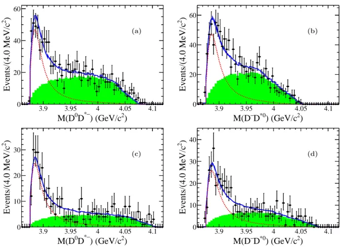
0 10 20 30 40 (d)FIG. 3. Simultaneous fits to the M (D ¯D∗) distributions of ((a) and (c)) π+D0D¯0-tagged and ((b) and (d)) π+D−D0-tagged processes for ((a) and (b)) data at√s=4.23 GeV and for ((c) and (d)) data at√s=4.26 GeV. The dots with error bars are data and the lines show the projection of the simultaneous fit to the data. The solid lines (blue) describe the total fits, the dashed lines (red) describe the signal shapes and the green areas describe the background shapes.
convolved with the mass resolution, and ǫ(mD ¯D∗) is the
reconstruction efficiency. The background PDF is pa-rameterized by phase space MC simulation. The sig-nal and background yields and the mass and width of Zc(3885)−are determined in the fit. The mass and width
of Zc(3885)−are constrained to be the same for both
pro-cesses.
A. Signal Term
The process e+e− → π+Z
c(3885)− with Zc(3885)−→
I is described with phase space generalized for the angular momentum L of the π+ − Z
c(3885)− system, where I
denotes D−D∗0 (labeled as a) and D0D∗− (labeled as
b). The Zc(3885)− is described by a mass dependent
width Breit-Wigner (MDBW) parameterization [35]. SI(mD ¯D∗) ∝ dN/dmD ¯D∗
∝ (κ∗)2L+1fL2(κ∗)|BWI(mD ¯D∗)|
2, (2)
where κ∗is the momentum of Z
c(3885)−in the e+e−rest
frame, fL(κ∗) is the Blatt-Weisskopf barrier factor [36],
BWI(mD ¯D∗) ∝ pmD ¯D∗ΓI m2 Zc− m 2 D ¯D∗− i 1 2mZc(Γa+ Γb) ,(3) ΓI = ΓZc[q ∗ I/q0I]2ℓ+1[mZc/mD ¯D∗][fℓ(qI∗)/fℓ(qI0)]2, qI∗ is
the D momentum in the Zc(3885)− rest frame, ℓ is the
angular momentum of the (DD∗)− system, and q0 I ≡
q∗
I(mZc). In the fit, mZc and ΓZc are free parameters,
while L = 0 and ℓ = 0 are fixed according to the analysis of angular distributions below. Parameters of the reso-lution and efficiency functions, obtained from MC and described below, are fixed in the fit.
B. Reconstruction Efficiency and Mass Resolution
In order to obtain the reconstruction efficiency and mass resolution, we generate a set of MC samples for e+e−→ π+Z−
c (Zc−→ (D ¯D∗)−), each with a fixed mass
value, zero width and JP = 1+ of the Z−
c , and subject
these MC samples to the same event selection criteria. The isospin channel e+e−→ π+D0D∗− (D∗− → D−π0)
can feed into the π+D−D0-tagged process. We
there-fore generate two corresponding MC samples by assum-ing the same decay branchassum-ing fraction between the pro-cess Z−
c → D−D∗0and Zc− → D0D∗−. The
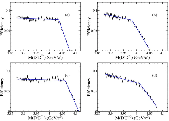
reconstruc-tion efficiency is estimated using the sum of the two MC samples, as shown in Fig. 4.
MC samples for e+e− → π+Z−
c (Zc− → (D ¯D∗)−) are
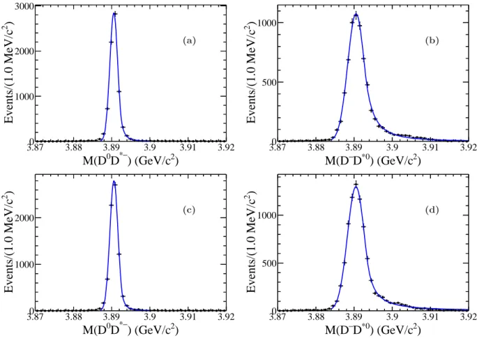
used to determine the mass resolution. The mass and width of Zc are set to be 3890 MeV/c2 and 0 MeV,
re-spectively. The mass resolution for the π+D0D¯0-tagged process is described by a Crystal Ball (CB) function [37]. Since the π+D−D0-tagged process contains two isospin
processes, the mass resolution is represented by a sum
of two CB functions with a common mean and differ-ent widths. The fit results for both processes are shown in Fig. 5. The resolution for the π+D0D¯0-tagged
pro-cess is determined by the fit to be 1.1±0.1 MeV/c2,
while the resolution for the π+D−D0-tagged process is
calculated to be 2.2±0.1 MeV/c2 using the equation
f1σ1+ (1 − f1)σ2, where σ1 and σ2 are the individual
widths of each of the two CB functions and f1 is the
fractional area of the first CB function.
C. Fit Results
As shown in Fig. 3, we perform a simultaneous fit to the M (D ¯D∗) distributions for the π+D0D¯0-tagged
and π+D−D0-tagged processes with √s=4.23 GeV and
√
s=4.26 GeV data samples. The statistical signifi-cance of Zc(3885)−, estimated by the difference of
log-likelihood values with and without signal terms in the fit, is greater than 10σ. The mass and width of Zc(3885)−
are fitted to be MZc(3885) = (3890.3±0.8) MeV/c 2 and
ΓZc(3885)= (31.5±3.3) MeV, where the errors are
statis-tical only. Since the resulting mass and width might be different from the actual resonance properties due to the parameterization function of Zc(3885), we
cal-culate the pole position (P = Mpole − iΓpole/2) of
Zc(3885) which is the complex number where the
de-nominator of BWI(mD ¯D∗) is zero, and regard Mpole
and Γpole as the final result. The corresponding pole
mass (Mpole) and width (Γpole) of Zc(3885) are Mpole
= (3881.7±1.6) MeV/c2 and Γ
pole = (26.6±2.0) MeV,
respectively.
D. Angular Distribution
The quantum number JP assignment for Z
c(3885)−
is investigated by examining the distribution of |cosθπ|,
where θπ is the π+ polar angle relative to the beam
di-rection in the center-of-mass frame. If JP = 1+, the
relative orbital angular momentum of the π+-Z
c(3885)−
system could be either S-wave or D-wave. If we neglect the small contribution of D-wave due to the closeness of the threshold, the |cosθπ| distribution is expected to be
flat. If JP = 0− (1−), the π+-Z
c(3885)− system occurs
via a P -wave and the |cosθπ| is expected to follow sin2θπ
(1+cos2θπ) distribution.
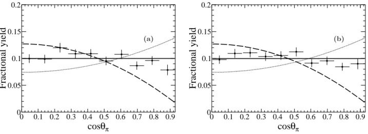
The |cosθπ| distribution of data is plotted with the
ef-ficiency corrected signal yield of combined data samples at√s=4.23 GeV and√s=4.26 GeV in ten |cosθπ| bins,
where the signal yields in different bin are extracted with the same simultaneous fit method described above. Figures 6 (a) and (b) show the |cosθπ| distribution for
π+D0D¯0-tagged process and π+D−D0-tagged process,
respectively. The data agrees well with the flat distribu-tion expected for JP = 1+ (χ2/NDF = 16.5/9 for the
π+D0D¯0-tagged process and 12.8/9 for the π+D−D0
distribu-)
2) (GeV/c
− *D
0M(D
3.85 3.9 3.95 4 4.05 4.1Efficiency
0 0.05 0.1 (a))
2) (GeV/c
*0D
−M(D
3.85 3.9 3.95 4 4.05 4.1Efficiency
0 0.05 0.1 (b))
2) (GeV/c
− *D
0M(D
3.85 3.9 3.95 4 4.05 4.1Efficiency
0 0.05 0.1 (c))
2) (GeV/c
*0D
−M(D
3.85 3.9 3.95 4 4.05 4.1Efficiency
0 0.05 0.1 (d)FIG. 4. Distributions of the efficiency versus M (D ¯D∗) for ((a) and (c)) π+D0D¯0-tagged and ((b) and (d)) π+D−D0-tagged processes at ((a) and (b))√s=4.23 GeV and ((c) and (d))√s=4.26 GeV. The dots with error bars are the efficiencies determined from MC. The curves show the fits with a piecewise linear function.
tion expected for JP = 0− (χ2/NDF = 103.1/9 for the
π+D0D¯0-tagged process and 104.9/9 for the π+D−D0
-tagged process) and JP = 1−(χ2/NDF = 106.3/9 for the
π+D0D¯0-tagged process and 104.9/9 for the π+D−D0
-tagged process), where NDF is the number of degrees of freedom in the fit.
E. Born Cross Section
For the π+D0D¯0-tagged process, the Born cross
sec-tion times the (D ¯D∗)− branching fraction of Z
c(3885)− (σ × Br) can be calculated by σ(e+e− → π±Zc(3885)∓) × Br(Zc(3885)∓→ (D ¯D∗)∓) = N L(1 + δr)(1 + δv)P i,jǫijBriBrjBr(D∗− → π−D¯0)I ,(4)
where N is the signal yield, L is the integrated lumi-nosity, ǫij is the signal efficiency for the π+D0D¯0-tagged
process listed in Table III of Appendix A, where the sub-scripts i, j = 0 . . . 3 denote the neutral D final state, Bri is the individual branching fraction for D decay
from PDG [32], the radiative correction factor (1 + δr)
is determined by the measurement of the line shape of σ(e+e− → πD ¯D∗) [23], the vacuum polarization factor
(1 + δv) is considered in the MC simulation [38] and I =
Br(Zc(3885)− → D0D∗−)/Br(Zc(3885)− → (D ¯D∗)−)
= 0.5, assuming isospin symmetry. The value of all above variables are listed in Table I.
Since the π+D−D0-tagged process contains two
pro-cesses of Zc(3885)− → D−D∗0 with D∗0 → π0D0
(la-beled as α) and Zc(3885)−→ D0D∗−with D∗−→ π0D−
(labeled as β), the Born cross section times the (D ¯D∗)−
branching fraction of Zc(3885)− can be given by
σ(e+e−→ π±Z c(3885)∓) × Br(Zc(3885)∓→ (D ¯D∗)∓) = N L(1 + δr)(1 + δv)(P i,jǫαijBriBrjBr(D∗0→ π0D0) +Pi,jǫ β ijBriBrjBr(D∗− → π0D−))I , (5)
)
2) (GeV/c
− *D
0M(D
3.87 3.88 3.89 3.9 3.91 3.92)
2Events/(1.0 MeV/c
0 1000 2000 3000 (a))
2) (GeV/c
*0D
−M(D
3.87 3.88 3.89 3.9 3.91 3.92)
2Events/(1.0 MeV/c
0 500 1000 (b))
2) (GeV/c
− *D
0M(D
3.87 3.88 3.89 3.9 3.91 3.92)
2Events/(1.0 MeV/c
0 1000 2000 (c))
2) (GeV/c
*0D
−M(D
3.87 3.88 3.89 3.9 3.91 3.92)
2Events/(1.0 MeV/c
0 500 1000 (d)FIG. 5. Fits to the mass resolution at 3890 MeV for ((a) and (c)) π+D0D¯0-tagged and ((b) and (d)) π+D−D0-tagged processes at ((a) and (b)) √s=4.23 GeV and ((c) and (d)) √s=4.26 GeV. The dots with error bars show the distributions of mass resolutions obtained from MC, the curves show the fits.
where ǫα ij and ǫ
β
ij are the signal efficiency for the two
π+D−D0-tagged processes, listed in Table IV and V
of Appendix A, the subscripts i and j denote the D−
and D0 final states, respectively, with i = A . . . F and j = 0 . . . 3, Br(D∗0 → π0D0) = (61.9±2.9)% and
Br(D∗− → π0D−) = (30.7±0.5)% [32]. The value of
all above variables are listed in Table I.
We also add a Zc(4020)−in the fit with mass and width
fixed to the BESIII measurement [19]. The fit prefers the presence of a Zc(4020)− with a statistical significance of
1.0σ. We determine the upper limit on σ × Br at the 90% confidence level (C.L.), where the probability den-sity function from the fit is smeared by a Gaussian func-tion with a standard deviafunc-tion of the relative systematic error in the σ × Br measurement. We obtain σ(e+e−→
π±Z
c(4020)∓) × Br(Zc(4020)∓ → (DD∗)∓) < 18 pb at
√
s=4.23 GeV and <15 pb at√s=4.26 GeV, respectively, at 90% C.L..
V. SYSTEMATIC UNCERTAINTIES
The systematic uncertainties for the pole mass and width of Zc(3885)−, and the product of Born cross
sec-tion times the (D ¯D∗)− branching fraction of Z
c(3885)−
(σ×Br) are described below and summarized in Table II. The total systematic uncertainty is obtained by summing all individual contributions in quadrature.
Beam Energy: In order to obtain the systematic uncer-tainty related to the beam energy, we repeat the whole analysis by varying the beam energy with ±1 MeV in the kinematic fit. The largest difference on the pole mass, width and the signal yields is taken as a systematic un-certainty.
Mass Calibration: The uncertainty from the mass cali-bration is estimated with the difference between the mea-sured and nominal D∗masses. We fit the D∗ mass
spec-tra calculated with the output momentum of the kine-matic fit described in the Sec. III after removing the D* mass constraint. The deviation of the resulting D∗mass
to the nominal values is found to be 0.84±0.16 MeV/c2.
The systematic uncertainty due to the mass calibration is taken to be 1.0 MeV/c2.
π
θ
cos
0 0.1 0.2 0.3 0.4 0.5 0.6 0.7 0.8 0.9Fractional yield
0 0.05 0.1 0.15 0.2 (a) πθ
cos
0 0.1 0.2 0.3 0.4 0.5 0.6 0.7 0.8 0.9Fractional yield
0 0.05 0.1 0.15 0.2 (b)FIG. 6. Fits to |cosθπ| distributions for (a) π+D0D¯0-tagged and (b) π+D−D0-tagged processes. The dots with error bars show
the combined data corrected for detection efficiency at √s=4.23 GeV and√s=4.26 GeV, the solid lines show the fits using JP = 1+ hypothesis, and the dashed and dotted curves are for the fits with JP= 0−and JP = 1−hypothesis, respectively.
TABLE I. Summary of the product of Born cross sections times the (D ¯D∗)−branching fraction of Z
c(3885)− (σ × Br), the
errors are statistical only.
π+D0D¯0-tagged process π+D−D0-tagged process 4.23 GeV 4.26 GeV 4.23 GeV 4.26 GeV N 384±30 207±18 418±34 239±22 L (pb−1) 1091.7 825.7 1091.7 825.7 1+δr 0.89 0.92 0.89 0.92 1+δv 1.056 1.054 1.056 1.054 σ× Br (pb) 147.5±11.5 109.2±9.7 136.6±11.0 107.5±9.7 L(1 + δr )(1 + δv
) : The integrated luminosities of the data samples are measured using large angle Bhabha events, with an estimated uncertainty of 1.0% [24]. The systematic uncertainty of the radiative correction factor is estimated by changing the parameters of the line shape of σ(e+e− → πD ¯D∗) within errors. We assign 4.6% as
the systematic uncertainty due to the radiative correction factor according to Ref. [23]. The systematic uncertainty of the vacuum polarization factor is 0.5% [38].
Signal shape: The systematic uncertainty associated with the Zc(3885)−signal shape is evaluated by repeating
the fit on the M (D ¯D∗) distribution with a mass constant
width BW line shape (MCBW, 1 m2
Zc−m 2
D ¯D∗−imZcΓZc
) for Zc(3885)−signal. The resulting difference to the nominal
results are taken as a systematic uncertainty.
Zc(4020)− signal The systematic uncertainty associated
with the possible existence of the Zc(4020)− in our data
is estimated by adding the Zc(4020)− in the fit. The
dif-ference of fit results is taken as a systematic uncertainty. Background shape: The systematic uncertainty due to the background shape is investigated by repeating the fit with function fbkg(mD ¯D∗) ∝ (mD ¯D∗ − Mmin)c(Mmax−
mD ¯D∗)d [23] for the background line shape, where Mmin
and Mmaxare the minimum and maximum kinematically
allowed masses, respectively, c and d are free parameters. The resulting difference to the nominal results is taken as a systematic uncertainty.
Fit bias: To assess a possible bias due to the fitting procedure, we generate 200 fully reconstructed data-size samples with the parameters set to the values (input val-ues) returned by the fit to data. Then we fit these sam-ples using the same procedures as we fit the data, and the resulting distribution of every fitted parameter with a Gaussian function. The difference between the mean value of Gaussian and the input value is taken as a sys-tematic uncertainty of the fit bias.
Signal region of DT: In order to obtain the systematic uncertainty related to the selection of the signal region of double D tag, we repeat the whole analysis by chang-ing the signal region in the M ( ¯D) versus M (D) plane from the nominal region to −15 < ∆ ˆM < 10 MeV/c2
(|∆M| < 30 MeV/c2) and −25 < ∆ ˆM < 20 MeV/c2
(|∆M| < 60 MeV/c2) for π+D0D¯0-tagged, and −14 <
∆ ˆM < 11 MeV/c2 (|∆M| < 28 MeV/c2) and −20 <
∆ ˆM < 17 MeV/c2 (|∆M| < 42 MeV/c2) for π+D−D0
-tagged processes. The largest difference of fit results is taken as a systematic uncertainty.
system-atic uncertainty for P
i,jǫijBriBrjBr(D∗− →
π−D¯0) and (P
i,jǫaijBriBrjBr(D∗0 → π0D0) +
P
i,jǫbijBriBrjBr(D∗− → π0D−)) as the efficiency
related systematic uncertainty for π+D0D¯0-tagged and π+D−D0-tagged processes, respectively. The
efficiency related systematic uncertainty includes the uncertainties from MC statistics, PID, tracking, π0
and K0
S reconstruction, kinematic fit, cross feed and
branching fractions of D and D∗ decay. The uncertainty
due to finite MC statistics is taken as the uncertainty of the signal efficiency. A systematic uncertainty of 1% is assigned to each track for the difference between data and simulation in tracking or PID [23]. For π0
reconstruction, the corresponding uncertainty is 3% per π0 [39]. For KS0 reconstruction, the corresponding
uncertainty is 4% per K0
S [40]. The uncertainty due to
the kinematic fit is estimated by applying the track-parameter corrections to the track helix track-parameters and the corresponding covariance matrix for all charged tracks to obtain improved agreement between data and MC simulation [41]. The difference between the obtained efficiencies with and without this correction is taken as the systematic uncertainty for the kinematic fit. The cross feed among different decay modes is estimated using the signal MC simulation as detailed in Tables VI–VIII of Appendix B. The systematic uncertainties for the branching fractions of D and D∗ decay are estimated by PDG [32]. A summary
of the systematic uncertainties for signal efficiency is listed in Tables VI–VIII of Appendix B. The total efficiency related systematic uncertainties are combined by considering the correlation of uncertainties between each decay channels.
VI. SUMMARY
In summary, based on the data samples of 1092 pb−1
taken at √s=4.23 GeV and 826 pb−1 taken at
√s=4.26 GeV, we perform a study of the process e+e− → π−(D ¯D∗)+ and confirm the existence of the
charged charmoniumlike state Zc(3885)−in the (D ¯D∗)−
system. The angular distribution of the π+− Z
c(3885)−
system is consistent with the expectation from a JP = 1+ quantum number assignment. We perform
a simultaneous fit to the (D ¯D∗)− mass spectra for
the two isospin processes of e+e− → π+D0D∗− and
e+e− → π+D−D∗0 using a mass-dependent Breit
Wigner function. The statistical significance of the Zc(3885) signal is greater than 10σ. The pole mass
and pole width of Zc(3885)− are determined to be
Mpole=(3881.7±1.6(stat.)±1.6(syst.)) MeV/c2 and
Γpole=(26.6±2.0(stat.)±2.1(syst.)) MeV, respectively.
The products of Born cross section and the D ¯D∗
branching fraction of Zc(3885)− for e+e− → π+D0D∗−
and e+e− → π+D−D∗0 are combined into a weighted
average [42]. For the data samples at√s=4.23 GeV, the result is σ(e+e− → π±Z
c(3885)∓) × Br(Zc(3885)∓ →
(DD∗)∓) = (141.6±7.9(stat.)±12.3(syst.)) pb.
For the √s=4.26 GeV data sample, the result is σ(e+e− → π±Z
c(3885)∓) × Br(Zc(3885)∓ → (DD∗)∓)
= (108.4±6.9(stat.)±8.8(syst.)) pb.
The pole mass and pole width of Zc(3885)− and
σ(e+e− → π±Z
c(3885)∓) × Br(Zc(3885)∓ → (DD∗)∓)
are consistent with but more precise than those of BE-SIII’s previous results [23], with significantly improved systematic uncertainties. The improvement in the re-sults obtained in this analysis is due to the fact that the double D tag technique and more D tag modes are used and two isospin processes e+e− → π−(D ¯D∗)+
are fitted simultaneously with datasets at √s = 4.23 and 4.26 GeV. This analysis only has ∼9% events in common with the ST analysis [23], so the two anal-yses are almost statistically independent and can be combined into a weighted average [43]. The combined pole mass and width are Mpole= (3882.2 ± 1.1(stat.) ±
1.5(syst.)) MeV/c2 and Γ
pole = (26.5 ± 1.7(stat.) ±
2.1(syst.)) MeV, respectively. The combined σ(e+e− →
π±Z
c(3885)∓) × Br(Zc(3885)∓ → (DD∗)∓) is (104.4 ±
4.8(stat.) ± 8.4(syst.)) pb at√s=4.26 GeV.
ACKNOWLEDGMENTS
The BESIII collaboration thanks the staff of BEPCII and the IHEP computing center for their strong support. This work is supported in part by Na-tional Key Basic Research Program of China under Contract No. 2015CB856700; National Natural Sci-ence Foundation of China (NSFC) under Contracts Nos. 10935007, 11075174, 11121092,11125525, 11235011, 11322544, 11335008, 11425524, 11475185; the Chinese Academy of Sciences (CAS) Large-Scale Scientific Facil-ity Program; the CAS Center for Excellence in Parti-cle Physics (CCEPP); the Collaborative Innovation Cen-ter for Particles and InCen-teractions (CICPI); Joint Large-Scale Scientific Facility Funds of the NSFC and CAS under Contracts Nos. 11179007, U1232201, U1332201; CAS under Contracts Nos. YW-N29, KJCX2-YW-N45; 100 Talents Program of CAS; National 1000 Talents Program of China; INPAC and Shanghai Key Laboratory for Particle Physics and Cosmology; German Research Foundation DFG under Contract No. Collab-orative Research Center CRC-1044; Istituto Nazionale di Fisica Nucleare, Italy; Ministry of Development of Turkey under Contract No. DPT2006K-120470; Russian Foundation for Basic Research under Contract No. 14-07-91152; The Swedish Resarch Council; U.S. Department of Energy under Contracts Nos. DE-FG02-04ER41291, DE-FG02-05ER41374, DE-SC0012069, DESC0010118; U.S. National Science Foundation; University of Gronin-gen (RuG) and the Helmholtzzentrum fuer Schwerionen-forschung GmbH (GSI), Darmstadt; WCU Program of National Research Foundation of Korea under Contract No. R32-2008-000-10155-0.
TABLE II. Summary of systematic uncertainties on the pole mass and pole width of the Zc(3885)−, and the product of Born
cross section times the (D ¯D∗)−branching fraction of Z
c(3885)−(σ × Br). The items noted with * are common uncertainties,
and other items are independent uncertainties.
Source ∆Mpole ∆Γpole
∆(σ×Br) σ×Br (%)
π+D0D¯0-tagged process π+D−D0-tagged process (MeV/c2) (MeV) 4.23 GeV 4.26 GeV 4.23 GeV 4.26 GeV
Beam Energy 1.0 1.6 3.3 3.0 4.9 3.4 Mass calibration 1.0 L(1 + δr)(1 + δv)* 4.7 4.7 4.7 4.7 Signal shape 0.1 0.1 0.1 0.1 0.1 0.1 Zc(4020)−Signal 0.4 1.0 2.9 2.0 2.8 3.9 Background shape 0.4 0.1 2.0 0.5 2.9 0.9 Fit bias 0.2 0.1 0.5 0.3 0.1 0.8 Signal region of DT 0.2 0.7 4.2 1.4 0.8 1.4 Efficiency related 8.3 8.3 7.9 7.9 Total 1.6 2.1 11.5 10.3 11.2 10.7
[1] B. Aubert et al. (BaBar Collaboration), Phys. Rev. Lett. 95, 142001 (2005).
[2] Q. He et al. (CLEO Collaboration), Phys. Rev. D 74, 091104(R) (2006).
[3] C. Z. Yuan et al. (Belle Collaboration), Phys. Rev. Lett. 99, 182004 (2007).
[4] T. Barnes, S. Godfrey, and E. S. Swanson, Phys. Rev. D 72, 054026 (2005).
[5] S. L. Zhu, Phys. Lett. B 625, 212 (2005).
[6] E. Kou and O. Pene, Phys. Lett. B 631, 164 (2005). [7] F. E. Close and P. R. Page, Phys. Lett. B 628, 215
(2005).
[8] S. K. Choi et al. (Belle Collaboration), Phys. Rev. Lett. 100, 142001 (2008).
[9] R. Mizuk et al. (Belle Collaboration), Phys. Rev. D 80, 031104 (2009).
[10] K. Chilikin et al. (Belle Collaboration), Phys. Rev. D 88, 074026 (2013).
[11] R. Mizuk et al. (Belle Collaboration), Phys. Rev. D 78, 072004 (2008).
[12] R. Aaij et al. (LHCb Collaboration), Phys. Rev. Lett. 112, 222002 (2014).
[13] B. Aubert et al. (BaBar Collaboration), Phys. Rev. D 79, 112001 (2009).
[14] J. P. Lees et al. (BaBar Collaboration), Phys. Rev. D 85, 052003 (2012).
[15] M. Ablikim et al. (BESIII Collaboration), Phys. Rev. Lett. 110, 252001 (2013).
[16] Z. Q. Liu et al. (Belle Collaboration), Phys. Rev. Lett. 110, 252002 (2013).
[17] T. Xiao, S. Dobbs, A. Tomaradze and K. K. Seth, Phys. Lett. B 727, 366 (2013).
[18] M. Ablikim et al. (BESIII Collaboration), arXiv:1506.06018v2[hep-ex].
[19] M. Ablikim et al. (BESIII Collaboration), Phys. Rev. Lett. 111, 242001 (2013).
[20] M. Ablikim et al. (BESIII Collaboration), Phys. Rev. Lett. 113, 212002 (2014).
[21] M. Ablikim et al. (BESIII Collaboration), Phys. Rev.
Lett. 112, 132001 (2014).
[22] M. Ablikim et al. (BESIII Collaboration), arXiv:1507.02404v2[hep-ex].
[23] M. Ablikim et al. (BESIII Collaboration), Phys. Rev. Lett. 112, 022001 (2014).
[24] M. Ablikim et al. (BESIII Collaboration), arXiv:1503.03408v1 [hep-ex].
[25] M. Ablikim et al. (BESIII Collaboration), Nucl. Instrum. Methods Phys. Res., Sect. A 614, 345 (2010).
[26] S. Agostinelli et al. (GEANT4 Collaboration), Nucl. In-strum. Methods Phys. Res., Sect. A 506, 250 (2003); Geant4 version: v09-03p0; Physics List simulation en-gine: BERT; Physics List engine packaging library: PACK 5.5.
[27] J. Allison et al., IEEE Trans. Nucl. Sci. 53, 270 (2006). [28] Z. Y. Deng et al., Chin. Phys. C 30, 371 (2006). S.
Agostinelli et al., Nucl. Instrum. Methods Phys. Res., Sect. A 506, 250 (2003).
[29] S. Jadach, B. F. L. Ward, and Z. Was, Comput. Phys. Commun. 130, 260 (2000); S. Jadach, B. F. L. Ward, and Z. Was, Phys. Rev. D 63, 113009 (2001).
[30] D. J. Lange, Nucl. Instrum. Methods Phys. Res., Sect. A 462, 152 (2001).
[31] R. G. Ping, Chin. Phys. C 32, 599 (2008).
[32] K. A. Olive et al. (Particle Data Group), Chin. Phys. C 38, 09001 (2014).
[33] J. C. Chen, G. S. Huang, X. R. Qi, D. H. Zhang, and Y. S. Zhu, Phys. Rev. D 62, 034003 (2000).
[34] M. Xu et al., Chin. Phys. C 33, 428 (2009).
[35] A. Abulencia et al. (CDF Collaboration), Phys. Rev. Lett. 96, 102002 (2006).
[36] J. M. Blatt and V. F. Weisskopf, Theoretical Nuclear Physics (John Wiley & Sons, New York, 1952).
[37] J. E. Gaiser, Charmonium Spectroscopy from Radiative Decays of the J/Psi and Psi-Prime, SLAC-R-255 (1982). [38] S. Actis et al., Eur. Phys. J. C 66, 585 (2010).
[39] M. Ablikim et al. (BESIII Collaboration), Phys. Rev. D 81, 052005 (2010).
87, 052005 (2013).
[41] M. Ablikim et al. (BESIII Collaboration), Phys. Rev. D 87, 012002 (2013).
[42] We calculate the combined mean value and combined un-certainty using the method given in G. D’Agostini, Nucl. Instrum. Methods Phys. Res., Sect. A 346, 306 (1994). The covariance error matrix is calculated according to the independent uncertainty (the statistical uncertainty and all independent systematical uncertainties in Table II added in quadrature) in each measurement and the com-mon systematic uncertainty listed in Table II between the two measurements.
[43] We calculate the combined mean value and combined un-certainty using the method given in Ref. [42]. The pole mass and width of two analyses don’t have common sys-tematic uncertainties, while the Born cross section has the common systematic uncertainties from L(1 + δr)(1 +
δv).
Appendix A: Signal Efficiency
The signal efficiency for π+D0D¯0-tagged process at
√
s=4.23 GeV and √s=4.26 GeV are listed Table III, while the signal efficiency for π+D−D0-tagged process
and its isospin channel are listed in Table IV and V.
Appendix B: The Efficiency Related Systematic Uncertainty
The systematic uncertainties for signal efficiency are listed in Table VI–VIII.
TABLE III. Signal efficiency ǫij (%) for π+Zc(3885)−(Zc(3885)−→ D0D∗−), D∗−→ π−D¯0, D0→ i, ¯D0→ j, where i and j
denote the neutral D final states: K−π+, K−π+π0, K−π+π+π−and K−π+π+π−π0 (labeled as 0, 1, 2, 3, respectively).
{i, j} 4.23 GeV 04.26 GeV 4.23 GeV14.26 GeV 4.23 GeV 24.26 GeV 4.23 GeV 4.26 GeV3 0 30.23±0.17 30.30±0.17 14.68±0.12 14.76±0.12 17.54±0.13 17.53±0.13 6.50±0.08 6.46±0.08 1 15.23±0.12 15.47±0.12 6.65±0.08 6.52±0.08 7.80±0.09 7.80±0.09 2.45±0.05 2.33±0.05 2 17.42±0.13 17.33±0.13 7.50±0.09 7.45±0.09 8.01±0.09 8.00±0.09 2.30±0.05 2.30±0.05 3 6.64±0.08 6.62±0.08 2.26±0.05 2.29±0.05 2.41±0.05 2.30±0.05 0.35±0.02 0.30±0.02
TABLE IV. Signal efficiencies ǫα
ijfor π+Zc(3885)−(Zc(3885)−→ D−D∗0), D∗0 → π0D0, D−→ i, D0 → j, where i denotes
the charged D final states: K+π−π−, K+π−π−π0, K0
Sπ−, KS0π−π0, KS0π+π−π−and K+K−π− (labeled as A, B, C, D, E
and F , respectively), and j denotes the neutral D final states: K−π+, K−π+π0, K−π+π+π−and K−π+π+π−π0 (labeled as
0, 1, 2, 3, respectively).
{i, j} 4.23 GeV 04.26 GeV 4.23 GeV14.26 GeV 4.23 GeV 24.26 GeV 4.23 GeV 4.26 GeV3 A 24.29±0.16 23.96±0.15 11.49±0.11 11.63±0.11 13.61±0.12 13.57±0.12 4.76±0.07 4.58±0.07 B 10.78±0.10 10.72±0.10 4.44±0.07 4.44±0.07 4.92±0.07 4.89±0.07 1.21±0.03 1.14±0.03 C 24.66±0.16 25.11±0.16 12.02±0.11 12.05±0.11 14.22±0.12 14.27±0.12 5.09±0.07 4.89±0.07 D 11.56±0.11 11.55±0.11 4.85±0.07 4.87±0.07 5.79±0.08 5.62±0.07 1.61±0.04 1.53±0.04 E 14.56±0.12 14.75±0.12 6.23±0.08 6.31±0.08 6.31±0.08 6.24±0.08 1.70±0.04 1.59±0.04 F 19.29±0.14 19.13±0.14 9.05±0.10 9.11±0.10 10.67±0.10 10.64±0.10 3.51±0.06 3.38±0.06
TABLE V. Signal efficiencies ǫβ ij for π
+Z
c(3885)−(Zc(3885)−→ D0D∗−), D∗−→ π0D−, D−→ i, D0→ j, where i and j are
described in the caption of Table IV.
{i, j} 4.23 GeV 04.26 GeV 4.23 GeV14.26 GeV 4.23 GeV 24.26 GeV 4.23 GeV 4.26 GeV3 A 23.57±0.15 23.65±0.15 11.32±0.11 11.42±0.11 13.22±0.11 13.09±0.11 4.75±0.07 4.68±0.07 B 10.83±0.10 10.49±0.10 4.34±0.07 4.34±0.07 4.86±0.07 4.76±0.07 1.17±0.03 1.16±0.03 C 24.51±0.16 24.37±0.16 11.94±0.11 11.91±0.11 13.98±0.12 13.87±0.12 4.96±0.07 4.93±0.07 D 11.34±0.11 11.30±0.11 4.68±0.07 4.83±0.07 5.67±0.08 5.46±0.07 1.58±0.04 1.47±0.04 E 14.04±0.12 14.17±0.12 6.19±0.08 6.04±0.08 6.11±0.08 6.08±0.08 1.60±0.04 1.52±0.04 F 18.89±0.14 18.79±0.14 9.03±0.10 9.08±0.10 10.42±0.10 10.37±0.10 3.35±0.06 3.44±0.06
TABLE VI. The systematic uncertainties for signal efficiency (%) for π+Zc(3885)−(Zc(3885)− → D0D∗−), D∗− →
π−D¯0, D0→ i, ¯D0→ j, where i and j are described in the caption of Table III.
{i, j} PID Tracking π0 4.23 GeV 4.26 GeV 4.23 GeV 4.26 GeV 4.23 GeV 4.26 GeV 4.23 GeV 4.26 GeVKinematic fit MC statistics Cross feed Total
{0, 0} 4 5 0 0.6 0.5 0.6 0.6 0.2 0.2 6.5 6.5 {0, 1} 4 5 3 0.6 0.3 0.8 0.8 0.1 0.1 7.1 7.1 {0, 2} 6 7 0 0.7 1.2 0.8 0.8 0.1 0.3 9.3 9.3 {0, 3} 6 7 3 1.2 0.9 1.2 1.2 0.2 0.0 9.8 9.8 {1, 0} 4 5 3 0.5 0.6 0.8 0.8 0.1 0.2 7.1 7.1 {1, 1} 4 5 6 0.7 0.5 1.2 1.2 0.1 0.0 8.9 8.9 {1, 2} 6 7 3 0.9 0.4 1.2 1.2 0.2 0.1 9.8 9.8 {1, 3} 6 7 6 0.8 0.6 2.1 2.1 0.1 0.0 11.2 11.2 {2, 0} 6 7 0 0.7 0.8 0.8 0.8 0.2 0.1 9.3 9.3 {2, 1} 6 7 3 0.6 0.5 1.1 1.1 0.1 0.1 9.8 9.8 {2, 2} 8 9 0 1.3 1.1 1.1 1.1 0.0 0.0 12.2 12.1 {2, 3} 8 9 3 0.5 1.1 2.0 2.1 2.0 2.9 12.7 13.0 {3, 0} 6 7 3 0.8 0.6 1.2 1.2 0.1 0.3 9.8 9.8 {3, 1} 6 7 6 0.6 0.9 2.0 2.1 0.0 0.1 11.2 11.2 {3, 2} 8 9 3 1.0 1.6 2.1 2.1 2.4 2.5 12.8 12.9 {3, 3} 8 9 6 0.9 1.0 5.4 5.8 0.0 0.0 14.5 14.7
TABLE VII. The systematic uncertainties for signal efficiency (%) for π+Z
c(3885)−(Zc(3885)− → D−D∗0), D∗0 →
π0D0, D−→ i, D0→ j, where i and j are described in the caption of Table IV.
{i, j} PID Tracking π0 K0 S
Kinematic fit MC statistics Cross feed Total 4.23 GeV 4.26 GeV 4.23 GeV 4.26 GeV 4.23 GeV 4.26 GeV 4.23 GeV 4.26 GeV
{A, 0} 5 6 0 0 0.3 0.4 0.6 0.6 0.3 0.4 7.9 7.9 {B, 0} 5 6 3 0 0.1 0.1 1.0 1.0 0.3 0.2 8.4 8.4 {C, 0} 3 4 0 4 0.2 0.2 0.6 0.6 0.4 0.3 6.5 6.4 {D, 0} 3 4 3 4 0.4 0.3 0.9 0.9 0.2 0.2 7.1 7.1 {E, 0} 5 6 0 4 0.7 0.5 0.8 0.8 0.1 0.1 8.8 8.8 {F , 0} 5 6 0 0 0.4 0.3 0.7 0.7 0.5 0.5 7.9 7.9 {A, 1} 5 6 3 0 0.3 0.6 0.9 0.9 0.1 0.1 8.4 8.4 {B, 1} 5 6 6 0 0.3 0.7 1.5 1.5 0.1 0.1 10.0 10.0 {C, 1} 3 4 3 4 0.4 0.3 0.9 0.9 0.2 0.2 7.1 7.1 {D, 1} 3 4 6 4 0.2 0.1 1.4 1.4 0.2 0.1 8.9 8.9 {E, 1} 5 6 3 4 0.9 0.8 1.3 1.3 0.3 0.5 9.4 9.4 {F , 1} 5 6 3 0 0.6 0.4 1.1 1.0 0.2 0.3 8.5 8.4 {A, 2} 7 8 0 0 0.6 1.0 0.9 0.9 0.2 0.1 10.7 10.7 {B, 2} 7 8 3 0 0.5 0.4 1.4 1.4 0.1 0.3 11.1 11.1 {C, 2} 5 6 0 4 0.4 0.6 0.8 0.8 0.2 0.0 8.8 8.8 {D, 2} 5 6 3 4 0.4 0.3 1.3 1.3 0.2 0.2 9.4 9.4 {E, 2} 7 8 0 4 1.0 1.2 1.3 1.3 0.0 0.0 11.5 11.5 {F , 2} 7 8 0 0 1.0 0.9 1.0 1.0 0.3 0.3 10.7 10.7 {A, 3} 7 8 3 0 0.9 1.0 1.4 1.5 1.2 2.0 11.2 11.4 {B, 3} 7 8 6 0 0.0 0.3 2.9 3.0 0.0 0.0 12.5 12.6 {C, 3} 5 6 3 4 1.1 0.7 1.4 1.4 0.3 1.0 9.4 9.5 {D, 3} 5 6 6 4 0.8 1.2 2.5 2.6 0.0 0.0 10.9 11.0 {E, 3} 7 8 3 4 1.2 1.6 2.4 2.5 0.0 0.0 12.1 12.1 {F , 3} 7 8 3 0 0.8 0.9 1.7 1.7 0.2 0.2 11.2 11.2
TABLE VIII. The systematic uncertainties for signal efficiency (%) for π+Z
c(3885)−(Zc(3885)− → D0D∗−), D∗− →
π0D−, D−→ i, D0 → j, where i and j are described in the caption of Table IV.
{i, j} PID Tracking π0 K0 S
Kinematic fit MC statistics Cross feed Total 4.23 GeV 4.26 GeV 4.23 GeV 4.26 GeV 4.23 GeV 4.26 GeV 4.23 GeV 4.26 GeV
{A, 0} 5 6 0 0 0.7 0.5 0.7 0.7 0.5 0.5 7.9 7.9 {B, 0} 5 6 3 0 0.4 0.2 1.0 1.0 0.2 0.3 8.4 8.4 {C, 0} 3 4 0 4 0.2 0.3 0.6 0.6 0.2 0.3 6.4 6.4 {D, 0} 3 4 3 4 0.2 0.2 0.9 0.9 0.3 0.3 7.1 7.1 {E, 0} 5 6 0 4 1.0 0.8 0.8 0.8 0.3 0.3 8.9 8.9 {F , 0} 5 6 0 0 0.4 0.5 0.7 0.7 0.4 0.5 7.9 7.9 {A, 1} 5 6 3 0 0.8 0.6 0.9 0.9 0.2 0.2 8.5 8.4 {B, 1} 5 6 6 0 0.5 0.3 1.5 1.5 0.1 0.0 10.0 10.0 {C, 1} 3 4 3 4 0.4 0.5 0.9 0.9 0.1 0.2 7.1 7.2 {D, 1} 3 4 6 4 0.4 0.2 1.5 1.4 0.1 0.1 8.9 8.9 {E, 1} 5 6 3 4 0.8 0.9 1.3 1.3 0.6 0.4 9.4 9.4 {F , 1} 5 6 3 0 0.6 0.7 1.1 1.0 0.3 0.3 8.5 8.5 {A, 2} 7 8 0 0 0.8 0.9 0.9 0.9 0.2 0.2 10.7 10.7 {B, 2} 7 8 3 0 1.1 0.5 1.4 1.5 0.2 0.2 11.2 11.2 {C, 2} 5 6 0 4 0.8 0.8 0.8 0.8 0.2 0.1 8.9 8.9 {D, 2} 5 6 3 4 0.6 0.4 1.3 1.4 0.3 0.3 9.4 9.4 {E, 2} 7 8 0 4 1.4 1.2 1.3 1.3 0.0 0.0 11.5 11.5 {F , 2} 7 8 0 0 1.1 1.1 1.0 1.0 0.3 0.3 10.7 10.7 {A, 3} 7 8 3 0 1.1 1.1 1.5 1.5 1.4 1.8 11.3 11.3 {B, 3} 7 8 6 0 1.3 0.1 2.9 2.9 0.0 0.0 12.6 12.6 {C, 3} 5 6 3 4 0.8 0.8 1.4 1.4 0.2 0.9 9.4 9.5 {D, 3} 5 6 6 4 0.1 0.4 2.5 2.6 0.0 0.0 10.9 11.0 {E, 3} 7 8 3 4 1.6 1.2 2.5 2.6 0.0 0.2 12.1 12.1 {F , 3} 7 8 3 0 0.6 1.0 1.7 1.7 0.2 0.2 11.2 11.2