Tú
■TST
f 3 9 Ğ P || ‘I* ІИ I г й Íi^ г é ^ ^ йщ Y ^ Н“ ÍÍ5 'Т ;іb i n 1 F İ İ L İ L İ
u t ^ mn î Qİ ji 2 % ñ é t b ¡ ü ü í
i *» ., ä ω- Λ « ■ *· J ^ iif . ,,;i j ¿ 4¿ J ^ r i.'-î ? .’# :►,» ¿ ft *, Я “Г; '> »< «< fl "t .·* jüWİ5 ^ ,іУ *îA *^vi ; ff : >‘î, i :;Y|« T Ij || w Du'4 (i«ÿ tt w àlifi Лй I Ö» ^ jU?
''^ЦЬУН:іΨ^-'ΊΙ -i ^ ú Ü-I-J
'<J w ^ w>‘w'-j( 'ij*^'.; 'C> - ..V··'
·,<·'.. * 'i y · ; ^ ;* . ._ ·>ν. f · · ' ;, ■. '^*'' ^►7 .^*T í : , ·' I..··* i v * ; · ^ '"
■•''w Y':^?<.v y ".' ’■'
4 ^ Î* •'»JÎ-W r ts ü tj/ ifc i « ' « ,И· e »
H' ;·! ·-> ':-y. ¿i V' 4^'·’y Y'ÿvi Y r;·;·
·> ·*;·.,ι «'·*·♦*. ^ li i!/ 'Uf' Ja* tí í i j й«я ¡(J m¡
fi Av.íi«·' .’; .:·',;ί
i|¿ W wW· U j -A ii;^ w · ·.(*('·** '-U v .í./iá * i . ; í i, . . - 'j j
CONTROLLER DESIGN FOR A TRAJECTORY
TRACKING MISSILE BY USING INVERSE
DYNAMICS METHOD
A THESIS
SUBMITTED TO THE ,DEPARTMENT OF ELECTRICAL AND ELECTRONICS ENGINEERING
AND THE INSTITUTE OF ENGINEERING AND SCIENCES OF BILKENT UNIVERSITY,
IN PARTIAL FULFILLMENT OF THE REQUIREMENTS FOR THE DEGREE OF
MASTER OF SCIENCE
By
Hiiseyin Tiirkoglii January 1996
^ J ? IZ
• ■ і Я
I certify that I have read this thesis and that in my opinion it is fully adequate, in scope and in quality, as a thesis for the degree of Master of Science.
Assoc. Prof. Dr. 0 . Morgul(P/incipal Advisor)
I certify that I have read this thesis and that in my opinion it is fully adequate, in scope and in quality, as a thesis for the degree of Master of Science.
Dr. Erol Sezer
I certify that I have read this thesis and that in my opinion it is fully adequate, in scope and in quality, as a thesis for the degree of Master of Science.
I? 5 .
Prof. Dr. A. B. Özgüler
Approved for the Institute of Engineering and Sciences:
Prof. Dr. M ehrn^Baray
ABSTRACT
CONTROLLER DESIGN FOR A TRAJECTORY
TRACKING MISSILE BY USING INVERSE
DYNAMICS METHOD
Hüseyin Türkoğiu
M .S . in Electrical and Electronics Engineering Advisor: Assoc. Prof. Dr. O. Morgül
January 1996
In this thesis, a controller for a missile desired to track a given trajectory is designed by using the nonlinear inverse dynarnics(NID) method. The nonlin ear dynamic equations describing the motion of the missile are linearized from input to the output by using the NID method without any need to the lineariz ing approximations as in the conventional linearizing method. Hence, designed controller for the linearized system stabilizes the nonlinear system over entire range of the operating points. Two approaches used in the controller design are presented in this thesis.
Keywords : Autopilot, guidance, missile, nonlinear systems, inverse dy namics, gain scheduling, two-time scale systems
ÖZET
T E R S D İN A M İ K Y Ö N T E M İ K U L L A N IL A R A K Y Ö R Ü N G E T A K İP E D E N B İR F Ü Z E İÇİN D E N E T L E Y İC İ T A S A R IM I
Hüseyin Türkoğlıı
Elektrik ve Elektronik Mühendisliği Bölümü Yüksek Lisans Danışm an: Assoc. Prof. Dr. Ö. Morgül
Ocak 1996
Bu tezde, doğrusal olmayan ters dinamik yöntemi kullanılarak yörünge takip eden bir füze için kontrol sistemi tasarlanmıştır. Bu yöntem kul lanılarak, klasik anlamdaki doğrusallaştırma yönteminde yapıları herhangi bir varsayıma gerek kalmadan, sistemin doğrusal olmayan girdi çıktı ilişkisi doğrusallaştırılmıştır. Dolayısıyla, tasarlanan doğrusal denetleyici, sistemi daha geniş bir alanda kontrol edebilmiştir. Denetleyici tasarımında kullanılan iki tür yaklaşım bu tezde anlatılmıştır.
Anahtar Kelimeler : Otopilot, güdüm, füze, doğrusal olmayan sistemler, ters dinamik, kazanç tablolaması, iki zamanlı sistemler.
ACKNOWLEDGMENTS
I would like to thank to Assoc. Prof. Dr. 0 . Morgiil for his supervi sion, guidance, suggestions and encouragement through the development of this thesis.
I would also like to thank to Prof. Dr. Erol Sezer and Prof. Dr. A. B. Özgüler for reading and commenting on the thesis.
It is a pleasure to express my thanks to all my friends for their valuable discussions and helps.
TABLE OF CON TEN TS
1 Introduction
1
2 The Equations of Motion 4
2.1 Coordinate System s... 4
2.2 Basic Dynamic Equations 6 2.2.1 Translational Dynamics 6 2.2.2 Rotational D yn am ics... 8
2..3 The Attitude of Missile with respect to the E a r t h ... 10
2.4 Transformation Between Coordinate F r a m e s ... 11
2.5 Kinematic E q u a tio n s... 12
2.6 Modeling of the Aerodynamic F o r c e s ... 13
2.7 Separation of The Equations of M o t io n ... 15
3 In p u t/O u tp u t ( I /O ) Linearization Using Inverse Dynamics M ethod 17 3.1 I/O Linearization P ro b le m ... 21
3.2 I/O Linearization of SISO Non-linear S y s te m s ... 22
3.3 Multi Input Multi Output (MIMO)Case 26 vi
4 The Use of Nonlinear Inverse Dynam ics(NID) Method in Con troller Design for Trajectory Tracking Missile 29
4.1 The First M e th o d ... 29 4.1.1 The Guidance Design by Using Inverse Dynamics Method 30 4.2 Acceleration Autopilot D e s ig n ... 36 4.3 Second M e t h o d ... 41
5 S IM U L A T IO N S 44
•5.1 The Simulation P rog ra m ... 44 5.2 Simulation R e s u l t s ... 46
6 C O N C L U S IO N 50
LIST OF FIGURES
2.1 Body F ra m e ... 6
2.2 Euler A n gles... 10
2.3 Angle of attack and sideslip a n g le ... 14
3.1 I/O linearization s c h e m e ... 22
3.2 State feedback with inverse dynamics 28 4.1 Guidance and A u t o p i l o t ... 30
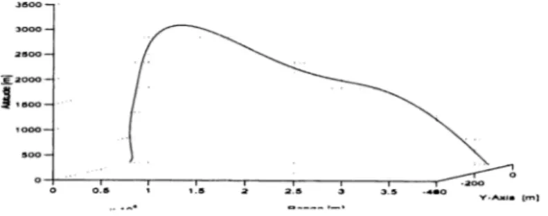
4.2 Autopilot Configuration 39 5.1 Desired tra jectory ... 46
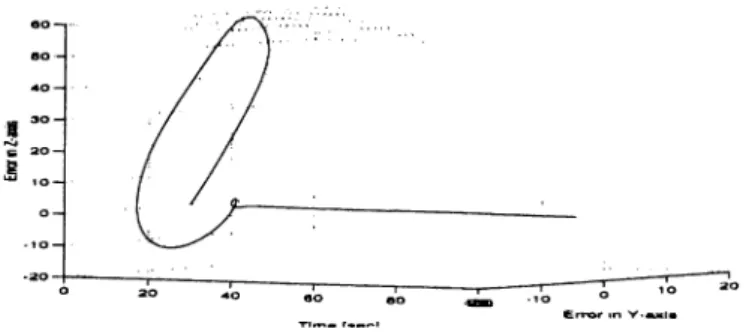
5.2 Position E r r o r ... 47
5.3 Angle of attack and Canard deflection 47 5.4 Desired trajectory for 6-DOF s im u la tio n ... 48
5.5 Position error for 6-DOF sim ulation... 49
5.6 Position errors in Y and Z axis 49 5.7 Position Error for Second M e th o d ... 49
5.8 Angle of Attack and Canard D eflection ... 49
Chapter 1
Introduction
All systems in the nature are nonlinear. Hence, analyzing and controlling these systems require deep understanding of the nonlinearity. This may not be obvious when we consider the linearized version of the nonlinear system. As long as the nonlinear system is in the vicinity of a chosen operating point, the designed linear controller for the linearized version of the nonlinear system at this operating point does its job. However, when the operating point of the system changes due to the external disturbance or some other reasons, the system may become unstable. For this reason, we have to develop a method to prevent this possibility. A straight-forward way of overcoming this problem may be ’’ gain scheduling m ethod”, [3], [4]. In this method, linear-time in variant controllers are designed for each linearized representation of the system at the selected operating points, so that the stability and certain performance objectives are achieved; these controllers are then linked together in order to obtain a single controller for the entire range of the system operation.
In between operating points, there is no guarantee that the system remains stable. Hence, extensive computer simulations are needed to validate the ro bustness of the controller designed by the gain scheduling technique. There are some heuristic rules-of-thumb in choosing the scheduling variable for the gain scheduling. The scheduling variable should vary slowly and capture the plant’s nonlinearity, [3].
Dynamic inversion method is another way of designing controllers for the nonlinear systems [1]. The nonlinear system may be transformed into in- put/output linear form by using this method without any approximations.
As a result, the designed nonlinear controller stabilizes the nonlinear system over the entire range o f operating points except for certain singular points. Nevertheless, this method requires the exact knowledge of the mathematical model of the nonlinear system. However, the exact modeling is not possible in practice. So, some robust control methods should be combined with this method, [6].
There are also some other nonlinear controller design techniques available. In [5], a nonlinear feedback law is derived for a nonlinear system by combining the linear controllers designed for a family of operating points. In [8], a partial dynamic inversion is proposed to overcome some difficulties in exact inversion theory. The model following approach is also a way of designing nonlinear controller, [13].
In this thesis, the controller for a trajectory tracking missile is designed by using dynamic inversion method with some modifications. The missile is controlled by using the four canards located on the surface of the missile. The deflection of canards has the effect of changing the aerodynamic forces and moments applied to the missile. Hence, the position of the missile can be controlled by deflecting the appropriate canard with a required deflection. The aim is to design a controller computing the required canard deflections so that the missile tracks a given trajectory.
Missile dynamics is composed of 12-state nonlinear dynamical equations. The derivation of these dynamical equations are presented in chapter 2. The modeling of the aerodynamic forces and moments are given in this chapter. For more details, see [9], [10], [11]·.
In chapter 3, the input/output(i/o) linearization ( dynamic inversion) method is presented. The second section considers only the nonlinear sin gle input single output(SISO) system. I/O linearization for multi input multi(MIMO) output case is explained in the third section. The more detailed analysis of these techniques can be found in [12].
In chapter 4, the controller design strategies for the trajectory tracking mis sile are presented. Two approaches used in controller design are given. The dynamics of the missile is separated into two parts as slow and fast dynam ics in the first approach. This method has been known as ” two-time scale
approach” and has been used in flight controller design for an aircraft, [2]. The two-time scale approach to the system resulted in order reduction, which
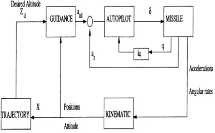
simplifies the controller design. In our case, the separated parts are controlled independently under certain constraints. For e.xarnple,the difference between speeds of the dynamics of these separated parts should be large enough. This rule puts some restriction on the dynamics of the controllers for these parts. The controller designed for the slow part is called as guidance unit, and the controller designed for the fast part is called autopilot unit. The guid ance unit computes the required acceleration for the missile to track the given trajectory. This computed acceleration is given to the autopilot as a reference command. The autopilot unit computes the required canard deflection to track the commanded acceleration.
In the guidance design, the dynamic inversion method is used. But critical model parameters have not appeared in the controller coefficients. Hence, the disadvantage of dynamic inversion method is avoided by using this approach. In autopilot design, the gain scheduling method is used.
In the second approach, the required canard deflection is directly found by using the dynamic inversion method. Hence, the gain scheduling technique is not used in this approach. Nevertheless, the critical model parameters ap peared in this controller algorithm. Since dynamic inversion method is based on the cancellation of the nonlinearity, any modeling error may cause unmod eled nonlinear dynamics. As a result of this, the controlled system may be unstable due to this unmodeled nonlinearity..
In chapter 5, the simulation results are presented and interpreted. In last chapter, the conclusions are given.
Chapter 2
The Equations of Motion
This chapter is devoted to the derivation of the mathematical equations de scribing the motion of a missile. The missile can be considered as a rigid body having a certain geometric structure for a stable flight. Derivation of the basic dynamic equations of a rigid body in six-degree-of-freedom (6-DOF) environ ment is based on the Newtonian Mechanics and can be found in standard text books on robotics or flight mechanics, see [9], [10], [11]. In these derivations, certain coordinate frames are defined. Hence, before getting into derivations of the motion equations, explanation of the coordinate frames used in derivations are presented.
2.1
Coordinate Systems
Any vector p in an n dimensional space R" can be represented in different ways depending on the chosen orthonormal basis for this space. Let X = be an orthonormal basis for R". The coordinates p with respect to are denoted [p]·’^ and are defined implicitly by the equation:
P =
! = 1
A' is also called as an orthonormal coordinate frame. It can easily be proven that kth coordinate of p with respect to X is given by
\p]^ = p · ^ '
where · denotes the inner product operation. Let E = and B = {6^, 6^, 6^} be two coordinate frames for R^. The representations of a vector
p & R? with respect to these coordinate frames are
\pf = p- p- p ■
[p]® = p ■ E p ■ E p · E
where superscript T denotes the transpose operation.
(2.L)
(
2
.2
)When a vector representation in one frame is given, the representation of the same vector with respect to other coordinate frame can be found by using a coordinate transformation. Coordinate transformation corresponds to a matrix multiplication
\pf = A[p]^ (2.3)
where the elements of the matrix A are Aij = E ■ E for ¿,j/' = 1,2,3. This matrix is orthogonal which is useful for calculations. Orthogonality of a matrix is expressed in mathematical form as
A -i = A^
In flight mechanics, certain coordinate frames are used depending on the controller design techniques. In the remaining part of this thesis, two coordi nate frame will be used. These are called as inertial frame and body frame.
The inertial reference frame is fixed in space. So it has no motion. But in practice, the frame fixed to the Earth is used as inertial frame, for the missiles flying over short ranges. For controller design, the difference between inertial and Earth frames are not so much. Hence, the Earth frame and inertial frame will be used interchangeable after this point. The direction of orthogonal axes X, Y, and Z of the Earth frame are as follows; X is directed to the north, Y is directed to the east and Z is directed to the center of the Earth.
The body frame( or body-fi.xed axis system) is attached to the missile such that its center is at the center of the gravity of the missile and rotates with it. In this coordinate frame, the axis OXb points to nose, OY^ points to right wing, and the axis OZb points down as shown in Figure (2.1). This coordinate frame will be denoted hy B = {i,j, A:} with z, j, k in the direction of OXi, 0Y6,
X
2.2
Basic Dynamic Equations
The mathematical equations describing the motion of a rigid body can be obtained by using the Newton’s second law of motion. It states that the change of momentum of a body is equal to the force applied on it. Mathematically, translational dynamic is described by
F = (2.4)
and rotational dynamic is described by
,7 ^^1 (2..5)
where F is the applied force, m is mass , Vt is total velocity of the object, M
is torque, and H is angular momentum. The symbol ]/ indicates the time rate of change with respect to the inertial frame.
2.2.1
Translational Dynamics
The equation (2.4), when the mass is assumed to be constant, can be rewritten as.
The time rate of change of velocity with respect to inertial frame can be ex panded as
d ^ d ^
(2.7) + w X Vt
-where Iv^is the unit vector along the total velocity vector, u is the total angular velocity. When the equation (2.7) is put in the equation (2.6), we have
F = m — (Vx)!^!, -\· Q X Vt (
2
.8
)Let the representation of the total translational and angular velocities of the missile in the body frame be
[VTf = {U ,V ,W ]
and
(u tI® = (?,?,!■ )
(2.9)
(
2
.
10
)
then the cross product of the vectors ujt and Vt becomes
uj X Vj = det
i j k p q r U V w
(
2
.11
)Here the determinant notation is used in a formal sense to indicate how to evaluate the cross product. In this case, the unit vectors {i,j,k} are treated as if they were scalars for the purpose of computing the determinant. When the equation (2.11) is expanded, we have
Q xVj· — i{qW - rV) + j{rU - pW ) + k{pV - qU) (2.12) The first term in right hand side of the equation (2.8) can be written as
— (Vr)lvr = iU + jV -t- kW
at (2.i;i)
When the representation of the total force in the body frame is taken as
[F T f = {F u F2,F s) (2.14)
the equation (2.8) can be rewritten by using equations (2.12), (2.13) as
= i{lf + W q - V r ) + j { V + U r - W p ) + k{W + V p -U q ) (2.15) 7
after equating the vector components of two sides and arranging certain terms, we have the following three translational dynamic equations.
IV
These equations can be written in a compact form as follows,
Fi — - Wq + VV m (2.16) F-2 — - U r + Wp rn (2.17) — - V p + Uq m (2.18) ’ u ' ' u ' ■ Eml ■ V = —w. V + Elm w w El _ m
-where w is a. skew symmetric matrix of the following form
(2.19) w = 0 —r <1 r 0 - p - 9 P 0 (
2
.20
)2.2.2
Rotational Dynamics
The same procedure used to derive the translational motion equations can be applied to the derivation of the angular motion equations. For a rigid body, angular momentum is defined as:
H = Iu
where I is inertia matrix of the form
(2.21)
/ = Ixy - h . — Ixy h III -ly x Iz (2
.22
)where Ix, ly, h denote moment of inertia terms , and Ixy, lx., ly. are product of inertia. For the symmetric missile under consideration, product of inertia terms are zero and ly = Iz- So the equation (2.22) has simplified form
/ =
0 0
0
ly
0
0 0 / ,(2.23)
Let the representation of the total angular momentum and torque on missile in the body frame be in the following forms,
[ M f = {7V4, My, /V/-}
(2.24) (2.25) By using the equations (2.24), and (2.23), the equation (2.21) can be rewrit ten as
■ H, ' pix
Hz =
. ^3 . T'lz
The rate of change of H with respect to the inertial frame is given by
| ( W ) ] , = 4 ( f f ) r „ ^ + i ; x ff (2.26) when the equation (2.21) is inserted in the equation (2.26), we obtain
+ ¿5 X / / (2.27) Hence, by using the equations (2.5) and (2.27), we have
M = / 4“ X H (2.28)
Note that u; x u5 = 0 is used in the last equation. Hence, when the right hand side of the equation (2.28) is expanded and when the components of each sides are equated, we have the following three angular motion equations:
9 = r = . M, ^ = T (2.29) My pr{Ix - L ) ly ly (2..30) ~~ ^y) Iz ~ h (2.31)
2.3
The Attitude of Missile with respect to
the Earth
The orientation of the missile with respect to the earth axes can be specified by using a set of angles called ’’ Euler angles” . These angles are depicted in Figure (2.2).
The definitions of these angles are,
$ is called as ’’ roll” angle which is between ON and 0Y6 axis measured in the OYbTjb plane
0 is called as ’’ pitch” angle which is between OX^ and the projection of OXfe axis on the horizontal plane including OX and OY axes.
'P is called as ” yaw” angle which is between OX and the projection of the
0X6 axis on the horizontal plane.
2.4
Transformation Between Coordinate Frames
It is well known that, any coordinate system can be obtained from any other one by a sequence of three rotations. Each rotation corresponds to a transfor mation matrix. The total transformation matrix is obtained by multiplication of these three matrices. The Euler angles are used in these sequence of rota tions. Let the inertial reference frame be denoted by E = {e i, e-2, e-}}.When the inertial frame is rotated around the vector by an angle't', corresponding transformation matrix will be,
m i =
cos('I') sin('P) 0
— sin('I’ ) cos('I') 0 (2.32)
0 0 1.
where coordinate frame Ei = {e^, e^, e.3} is rotated version of the inertial frame
E = {61,62,63}. When the frame E\ is rotated around e-2 vector by an angle
0 , resulting transformation matrix is of the form.
m i ; =
cos(0) 0 — sin(0)
0 1 0 (2.33)
sin(0) 0 cos(0)
where E2 = {61,62,63} is new frame. When this new frame is rotated about
the vector e[ by an angle $ , corresponding transformation matrix is
\T]t =
1
0
0
0 cos($) sin($) (2.34)
0 — sin($) cos($)
where resulted coordinate frame E3 = {61,62,63} is body frame B = {¿ ,j, ¿ }.
The overall transformation matrix is found by multiplication of these tunda- mental rotation matrices as [T\% = [T]|^.[r]|*[T]f,. When this multiplication is done, transformation matrix from inertial frame to body frame is found to be
C0C'P cG s'f —50
[ r ] f = 5^50c'{' — C$5'P 5 $ 5 0 5 ^ + 5$C0 (2.35) C<&50C'^ + C$505'& - 5<&CVt C^C0
The transformation matrix from the body frame to the Earth frame is just the transpose of the matrix given above
[7’]f =
C 0 C 'P S $ 5 0 C ' I ' - C $ 5 'P C < & S 0 C 'i' + 5 $ 5 ^
C05't S<I^505'I' + C^C'i C$S05'P — 5$C'P (2.36) —5 0 5<&C0 C$C0
where c denotes cosine and s denotes sine of the angle. Afterwards, the notation for the transformation matri.x given by (2.36) will be used without superscript or subscript, T = [T]g.
2.5
Kinematic Equations
The position and the attitude of the missile with respect to the inertial frame are found by solving the kinematic equations given in this section. Transla tional kinematic equations are as follows
■ a: ' ‘ u '
Y = T. V
z w
(2.37)
where X , V, and Z are the position components of the missile in the inertial frame along corresponding axes.
Since T is transformation matrix, it is orthonormal. Hence we can write the following
or
where /3 is 3 x 3 identity matrix. When time derivatives of the both sides of the equation (2.39) are taken, we have
(TT^) + = 0 (2.40) 12
2 ^ - 1__r p T (2. : !8)
which requires that TT^ is a skew-symmetric matrix.
TT^ = w
where w is given by the equation (2.20).
(2.41)
When we use the equations (2.41) and (2.20), we can obtain the following kinematic equations,
Q = q cos — r sin
$ = p + 9 sin($) tan(0) r cos(<&) tan(0) • sin(<]&) cos($)
cos(0 ) cos(0 )
(2.42) (2.43) (2.44)
These equations can also be obtained by geometric projections of angular rate vectors to corresponding axes.
The angular velocities p, q, and r are measured by three rate gyros located on yhe missile and used to find Euler angles by using the above equations.
2.6
Modeling of the Aerodynamic Forces
The external forces and torques on the missile may come from different sources such as thrust, wind, and aerodynamic forces. The total external force can be written as
Fx = i{Fj; + Tj, -b mçx) + j{Fy + Ty + f^Qy) + k(^F~ + + i^gz) (2.45)
where m is mass of the missile, Fx,Fy,F, are aerodynamic force components.
Tx,Ty,T, is thrust force components and py, p^ are gravitational accelera tion components along the body axes, ^he aerodynamic forces and moments applied on the missile are function of some flight parameters such as angle of attack(a), side slip angle(/?), mach number(M), air density(p), tempera- ture(T), angular rates (p, p, r) etc.The explanations of these flight parameters are given below.
Angle of attack and side slip angles specify the orientation of the missile velocity (Vt) with respect to the body axes as shown in the Figure (2.3)
The expressions of angle of attack and side slip angle are as follows IV 0! = arctan( — ) (2.46) and V [i = arctan( — ) Vt (2.47)
When IV and are small compared with f/’, which is acceptable , angle of attack can be approximated as
u
and side slip angle is approximated as
V
(2.48)
(2.49)
O
u
Figure 2..3: Angle of attack and sideslip angle
Mach number is defined as the ratio of the missile’s velocity to the velocity of the sound
M =
Y
l
c
where speed of the sound is
_ { ^kRTo[\ - 0.00002256/i] for h < 10000 m I \/7i.7744.kR.To for h > 10000 m The form of aerodynamic forces and moments are
■ F , ' ' c / F y = Q d ^ C y . . (2..50) (2.51) (2.52) 14
and
■ C l '
M y = Q d A d
Mz
. .(2.53)
where d is missile diameter, A is the missile cross sectional area, Qd is dynamic pressure. The dynamic pressure is defined as
1
Qd
— (2.54)where p is the air density depending on altitude(/i) in the following way.
P =
Po[l - 0.00002256/1]'*·'^·^® for h < 10000 m
for h > 10000 m (2.55) The terms Cy, C-, C'«, C/ in the equations (2.52) and (2.53) are the dimensionless aerodynamic force and moment coefficients. These coefficients are dependent on the flight parameters A/, a, /?, S, q, r etc.
2.7
Separation of The Equations of Motion
There are twelve non-linear differential equations completely describing the motion of the missile. However, under certain assumptions, some equations may be separated from others.
When the missile is assumed to move in only the pitch plane(such that = 0 ,r = 0, K = 0 ), and without any rotating motion (so that $ = 0, P = 0), si.x dynamic equations are reduced to three dynamic equations with the following form. i l = - ^ - W q + g, m W = E ± ^ U q + g, m
.
M,.
(2.56) (2.57) (2.58)Kinematic equations for pitch plane motion are, 15
where Tm is of the form, and Z = T — J- rr U w (2.59) T -^ m — C0 .S0 —S0 C0 e = q
(2.60)
(2.61)
When the missile is assumed to move in only the yaw plane(such that 0 = 0, <7 = 0, W = 0 ), and without any rotating motion (so that $ = 0, P = 0), the equations of motion will be
U = -^ + Vr + g, m V = ^ - U r + gy m r = M l L (2.62) (2.63) (2.64) Y = Trm y
u
V' ^ m y - s ^ (2.65) (2.66) ^ = r (2.67) 16Chapter 3
Input/Output (I/O )
Linearization Using Inverse
Dynamics Method
A nonlinear system may be transformed into a i/o linear form by means of a nonlinear state feedback. When such a nonlinear state feedback is found, the resulting system will be i/o linear and the linear controller design methods can be used without any need to linearization approximations as in the conventional linearization method. This approach has found a lot of applications in certain areas with some special modifications.
The basic idea in i/o linearization is to differentiate the output function with respect to time as many times as required until the input term appears in the equations. Then, provided that the coefficient matrix multiplying the input term is nonsingular, this equation may be used to obtain linear and decoupled equations between the output and a new reference input vectors. To illustrate this idea, for simplicity, let us consider a single input single output (SISO) linear system:
X = Ax + 6u, y — cx (3.1) where x ^ BA. The time derivative of the output is
y = cx = cAx + cbu (3.2) Let V be a reference input. If the coefficient {ch) multiplying the input term
(u) is nonzero, we choose the input as following
V— cAx u =
cb (3.3)
otherwise {cb = 0), we continue differentiation of the output until we have the input term. Let r be the order of differentiation required to have the input term. Then we have
= cA^x + cA^-%u (3.4)
where cA''~^b ^ 0. When we choose the input as
V — cA^x u =
cA^-^b
we have the following i/o relation, which is linear.
= u
(3.5)
(3.6)
The finite number of differentiation of the output required to have an input term is called relative degree and it is less than the dimension of the system. This fact can be easily proven for the linear SISO system (3.1). Let us assume that the relative degree r is greater than or equal to the system dimension n. Then we have
cA'b = Q fo r i = 0,1, ...,n — l,n , ...,r — 1 (3.7) We can deduce from the equation (3.7) by using the Cayley-Hamilton theorem that
cA‘ b = 0 for i = 0, i , ..., oo (3.8) This contradicts the definition of the relative degree. Hence, the relative degree is always less than the dimension of the system.
It can be shown that, when the relative degree is r, the vectors {c, cA, ..., cA'·“ ^} are linearly independent. Moreover, one can find the vectors
[hr+i, hr+2,···, hn} such that the set {c, cA, ..., cA’'~\ /ir+2,..., hn) is
linearly independent and < hi, 6 > = 0 i = r + 1 , .., n. With the new coordinates = cA '“ ^x j = 1,2, ...,r
Zj = hjX j = r + l , . . . , n
and the control law (3.5), state equations in the new variables become Zi — Z2 Z2 = Z3 (3.9) Zr = V -- ^ur^O d“ ^rr'^U y =
where Zo = [zi, Z2^ ...,2r]S z^ = [2^+1, Clearly, z^, denotes the unob
servable states. Moreover, for stability, obviously Arr must be a stable matrix. The dynamics given by
Zu = ArrZu (3.10) is called "zero dynamics” .
Fact. Let the transfer function of the linear system have the following form
(3.11)
G{s) = c{s l - A ) - 4 = d{s)
The zeros of the system, i.e. z such that п(дг) = 0, are eigenvalues of the closed loop system matrix (3.10).
Proof. For a system with relative degree one, closed loop system matrix can be written by inserting the input term (3.3) into the equation (3.1). The resulting closed loop system matrix is found to be
(.Э.12)
If is the zero of the system (3.1), it satisfies the following equations
Axo + buo = zXo (-^-LB)
CXo = 0
When we multiply the equation (3.13) by the output matrix c from left, we have
cA xo-{■ cbuo = ^ (3-14)
the input term Uo is found from the equation (3.14) as Uo = —^ Xq. When we put this input term into the equation (3.13)
AqXq — ZX(^
19
where Ac is the closed loop state matrix given by (3.12). We can see from the equation (3.15) that the zeros of the system are the eigenvalues of the closed loop system matrix Ac- Suppose that the relative degree r is greater than one. In this case, when we put the computed input (3.5) into the system equation (3.1), we have
V X = ( I---)Ax + b
---^ cA^-^h’ cA’- ‘ 6 So closed loop matrix has the expression
(3.16)
cA'-^b'
When we multiply the equation (3.13) by the term c.4'’~‘ from the left, we have
cA^'xo + cA’’~''buo = cA''~^~Xc (•^•J-7) Note that right-hand side of the equation (3.17) is zero. In order to see this fact, we use the expression of Axo given by (3.13)
cA'' ^zxo = zcA'' ^{Axo) = zcA’’ {zxo — buo) = z'^cA’’ ^x (3.18) Note that, due to the definition of the relative degree, cA’’ ^buo = 0. By this way, we can proceed as follows
cA^ ^zXo z^cA'’ ^Xo = ... = z'^cXq = 0 Hence, we can rewrite the equation (3.17) as
cA^Xo + cA^~^buo = 0
When we extract the input term Uo and put it into (3.13), we have
Ac Xo = ZXo
(3.19)
(3.20) where Ac is given by (3.16). Hence, s is an eigenvalue of the closed loop system matrix. So, the proof is completed.□
The alternative way of seeing this fact is the following. Suppose that the system has a relative degree of r. In Laplace domain, we can write the relation between the reference input and the output of the system by using the equation (3.6) as
n ‘ ) = ^ = G(s)U{s) = ^ £ / ( s )
So, we have the following dynamics(transfer function) in the input generation process
U(s) q(s)
^ ' (3.21)
V{s) p{s)s’’
As a result of this fact, when the system given by (3.1) has zeros on the right-half complex plane (has unstable zeros), the zero dynamics of the closed loop system will be unstable. Because, unstable zeros of the open system turn out to be the eigenvalues of the zero dynamics. Consequently, inverse dynamics method can not be applied to the control of the non-minimum phase systems. This fact can be applied to the nonlinear systems also. In that case, definition of the poles and zeros of the system are modified in an appropriate way. More detailed analysis of this fact can be found in [12]
3.1
I /O Linearization Problem
Let the non-linear system be described by the following state and output equa tions
m
X = f { x ) + J2gi{x)ui ,i= l..m (3.22)
i
y = h{x) (3.23)
where x £ is the state vector; y € R™ is output vector; f : R’^, Qi : R”· R^, and h : RP· RT" are vector fields.
The i/o linearization problem can be stated as follows;
I / O L inearization P r o b le m : Find a state control law of the form
V = q{x) + S{x)u, (3.24)
where q{x) G and S{x) G R”^^^ smooth functions of x, such that the new input-output relationship is in the following form
d f' - Vi, i - l..r/i, (3.25)
which means that i** channel is decoupled from other channels and i/o relation at each channel is linear.
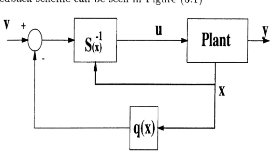
This feedback scheme can be seen in F’igure (3.1)
Figure 3.1: I/O linearization scheme
3.2
I /O Linearization of SISO Non-linear
Systems
Let us consider the single-input, single-output(SISO) nonlinear system de scribed by the following state equations,
X = f { x ) + g{x)u, y = h{x) (3.26) The following definition will be used in the subsequent derivations .
Lie D eriva tive: Let h \ R and / : ^ /2” be smooth functions. The map
is called as the Lie Derivative of the function h with respect to the vector field / , and denoted by Ljh. The kth order Lie derivative is defined recursively as
L)h = Li{L)-^h)
The time derivative of the output in the equation (3.26) is
y — (^/^)(x) T (3.27)
Let us assume that there exists e > 0 such that
(La/i)(i) 0 / o r X e BJ^Xo) = {a: : ||a; - < e,a: € /?” } (3.28) We define the functions q{x) and S{;x) in the equation (3.24) as,
^(x) = *^(^) — i^gh)(x) (3.29) so that when we choose the input to the system as,
0 - q{x) u =
S{x) (3.30)
we obtain the following linear relation between the reference input (u) and the output of the system (3.26) in the ball defined in (3.28)
y = v
Suppose that we can not find a ball B^{xo) for any e such that (Lgh)(^.j.) ^0
for all X € Be. Hence, the required input can not be found from the equation (3.30). Let us suppose that derivative of the output is in the following form.
such that
{LgL’jh)(^^) = 0 , k = 0 , l , . . , r - 2
{LgLy^h)(.,)^0
for X € Be. Then the reference input can be defined as
V = (Ly/i)(^) + u{LgUj ^/i)(x)
When we extract the input term from the equation (3.34), we have ^ V - (L^/t)(x) “ (LgUf^h\,) (3.31) (3.32) (3.33) (3.34) (3.35) When we apply this input to the nonlinear system, we have the following i/o relation
yi-·) = u (3.36)
It can be shown that, the relative degree (r) is less than the dimension of the system, see[12]. Let us define the following new state variables
Zi = L\~^h{x) ¿ = 1,2, ..., r
Zg = ipj{x) j = r + l,...,n
such that
= 0 i = r + l , . . . , n where ^j{x) are smooth functions of x and the set
d[jjhj{^x^^ dtLjfi(^x'^<f »»,y dL·j hl^x'j^ dip/'^i^ d(pj<^21 *··? d ^ ji} (3.*5T)
a,t X = Xo is independent. The state equations in the new variables with the control law (3.35) become
~1 = ^2 ¿2 = 23 (3.38) ir = n Zu = $ (2o ,2„) = $i(o;) y = Zi
where i>l(x) = [Z//</?r+l, Lf(fr+2, ■■■■, Lj(pnV, Zo = [zi, Z2, ...,2r]^, Zu =
[zr+i, ....,2:„]^. Clearly, Zu denotes the unobservable states. The dynamics given by
iu = $ (0 ,z „) (3.39) is called "zero dynamics” of the SISO nonlinear system (3.26), and should be stable for application of the NID law in stabilization of the nonlinear system. The following example illustrates application of the NID law to i/o linearize a nonlinear system.
Example. Let us take the SISO non-linear system described by equations
(3.26) with.
X2 ’ 0 ‘
/( ^ ) = Xl T XiX2 , gi x) = 1 2xi -1- X2 0
, /l ( X ) X3 (:i.40)
we have the following Lie derivatives
(Lj/l)(a;) — 2xi -f X'2, iLg^)(x) 0
{L^jh)(x) — 2x2 + xi + X1X2, {LgLfh)^x'^ = 1
So the relative degree (r) of this system is 2. When we choose the following new state variables
zi = h{x) — X3
~2 — (^ /^ )(^ ) — —2xi + X2
^3 = <^3(3;) = a:i + X2
and the input as
u = V + 2xi — xi — X1.X2
vve have the following new state equations it = Z2
¿2 - V
¿3 = -2^1 + 2z2 + 2^3
y = zi
Note that, the zero dynamics of this closed loop system described by the fol lowing equation is unstable.
¿ 3 = 2z3 (3.41)
When we linearize the system about the equilibrium point (xi,ar2,X3) = (0,0.0) , we have u 0 1 0 ' ' 0 ' X = 1 0 0 X + 1 - 2 1 0 _ 0 y = 0 0 1 ] X
where x = [xi X2 X3Y ■ The transfer function of the linearized system is
G{s) = s - 2
s(s^ — 1)
Note that the zero of the open loop system is unstable, which becomes the eigenvalue of the zero dynamics (3.41). Hence, we can not use the NID law to control this system.
Note that, when the linearized version of the system about an equilibrium point has an unstable zero, NID law can not be applied to the nonlinear system to stabilize it about that equilibrium point. However, this condition gives only the necessary but not sufficient condition for the application of the NID law. In other words, showing that linearized system does not have any unstable zero is not sufficient to use NID law.
3.3
Multi Input Multi Output (M IM O )Case
The same method (used in SISO case) with minor modifications can be used in MIMO case. First the definition of the relative degree is slightly different. It is not a scalar but a vector of the form
r = '■i ^2 such that
= 0, A: = 0 , l , . . . , ( r . - 2 ) and the matri.x 5 (x ) of the form
(3.42)
(3.43)
S = {^31^^/ ^^2)(x) {^32^y ^^2)(i)
('^51·^/"* ^m){x) (^52·^/”* hm){x) [Lg^^Lj^ *^m)(o,·)
(3.44)
which is non singular in the ball about an operating point x^. By defining
9 as a vector with elements,
qг = L]'h,, (3.45) the resulting i/o relation of the system (3.22) with the new reference input defined in (3.24) becomes in the form (3.25). The proof of the followin theorem can be found in [12].
Theorem. 1. Suppose the system (3.22), (3.23) has relative degree vector r as in (3.42) with rd — Z)i^i(ri). Then there exists a local diffeomorphism T around Xo, such that, in terms of the new state vectors 2 = T’(x), and with the reference input v , the system dynamics is described by
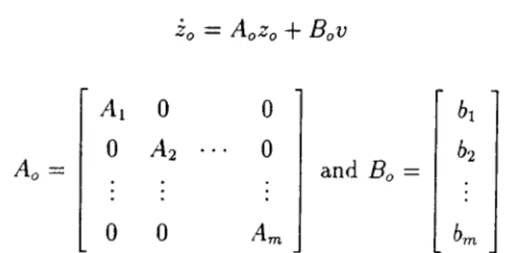
1
dt -2 ^1 where Zi ■ i — 1,2, ..,m , Zu € /2" = ^1 0 0 r n 61 ■ 0 ■ 0 A2 0 b-z 0 ^2 + u+ 0 0 0 b-m 0 0 0 0 0 _ 1 _ Vl = ^¿,li i ■= 1,2, ^¿,2 ~i,r. r e R"·, bi= 0 0 1 (/u (-)+ y~ l <7u;(~)t’;') J = l (3.46) 6 for 6 Z2™ is the reference Vl V2 · · · v,ninput vector, and A{ is a r,· x r, matrix with the following form(cornpanion form). ’’ 0 1 0 0 0 A = 0 0 1
0
0
0
0
1
0 0 0 0The transformed system equations (3.46) can be partitioned as,
Z,· = A{Zl T Hi — QZ;, I 1, 2, ...^Tn
and
(3.47)
(3.48)
•2u — fu{z) + '^9uj{z)Vj (3.49)
i=l
Note that states Zu are not observable and does not have any effect on other states.
Definition.(Zero Dynamics for M IM O nonlinear system)
Let the transformed state vector z be partitioned as z = [z^ z„]^, then the following dynamic equation is called the zero dynamics of the system (3.46),
¿u = /u (0 ,z„) (3.50) Clearly, z^ denotes the observable states, and z„ denotes the unobservable states of the system. The observable states are evolved by the following dynamic
equation where Zq — ÆqZq “f· BqV (3.51) 0 0 ' 61 ■ 0 A2 · ■·· 0 and Bo = ^2 0 0 /lo =
If the zero dynamics of the system is stable, the observable part of the sys tem can be stabilized by using certain linear controller design techniques. For example, we can use the following state feedback
u = - K z .
to stabilize the system. When we apply this outer-loop control, the closed loop system matrix will be A, = Ao — BqK· Since the system (3.51) is controllable, we can place the poles of the closed loop system at any place in the complex plane. This stabilization scheme is depicted in Figure (3.2)
Figure 3.2: State feedback with inverse dynamics
Second part called as autopilot unit operates on fast dynamics and com putes the required canard deflection to achieve the commanded acceleration computed in the guidance unit. This part is designed by using conventional controller design technique. The overall controller structure is shown in the Figure (4.1)
4.1.1
The Guidance Design by Using Inverse Dynamics
Method
In this subsection, the guidance algorithm is derived by using the nonlinear inverse dynamics method . The problem is to design a guidance unit comput ing the required acceleration so that when the missile tracks this computed acceleration, it also tracks a given trajectory .
Figure 4.1: Guidance and Autopilot
The derivation of the guidance law for the pitch plane is presented first. .After that, the full formulation for guidance law is presented, in which case, all the equations of motion of the missile are taken into account without any assumption.
The Guidance Law for Pitch Plane.
The motion of the missile in the pitch plane is described by the equations (2.56), (2.57), (2.58), (2.59), and (2.61). In the sequel, pitch and yaw motions
are assumed to be decoupled. If the motion in yaw plane is small and there is no rolling motion, this assumption may be valid.
Let the desired trajectory be given in the following form,
Z, = f { X ) (4.1)
where / is continuous, double differentiable function of X , cind is the desired altitude of the missile at X. The position error is defined as.
e = Z - Zd
The first derivative of the error with respect to time is.
(4.2) · or e = ’ X ' 11 ax ^ J Z
when the eciuation (2.59) are inserted in (4.3), we obtain
¿ = GT,r U w
where G is defined as
G = ax ^1
(4.3)
and Tm is the transformation matrix given by (2.60). The second time deriva tive of error is.
(4.4) Since Tm is transformation matrix, its derivative with respect to time can be written as. ' U ' ' u ' + GTm ' u ' ’¿ = GTm + GTm w W w Tm = TmW 31 (4.5)
where w is skew-symmetric matrix with the following form,
w = 0 q
- q 0 Also noting that,
U w —w
u
w
+ Fxfm F,/mso the equation (4.4) can be rewritten as,
= GTm Fx/m -f- gx
FJm + gy S ' « · (4.6)
Let r be reference input. When we equate second time derivative of the error (4.2) to this reference input,
e = r (4.7)
then the aerodynamic acceleration (a,) in Z direction {F^/m) is found to be p _ [('^ - q) + + (I x cos(Q) + sin(0))g^
(cos(0 ) - | ¿ s in (0 )) If the reference input is chosen as.
r = —kdt — kpe (4.9) then the following second order linear differential equation describing the error dynamic can be found by using (4.7) and (4.9),
e + kde + kpe = 0 (4.10)
where the parameters kj, and kp are real positive numbers and found with respect to the desired error dynamics. By inserting the equation (4.9) into the equation (4.8), desired acceleration is found to be
_ [j-kde - kpt - g ) + ^ j X ) ^ ] + (|^ co s(0 ) + sin(0))a^ (cos(0 ) - | ^ sin (0 ))
This acceleration is given to the autopilot unit as acceleration command.
In the equation (4.11), singularity problem arises when denominator equals to zero. If the denominator is equated to zero, we have
(4.12) This situation occurs when the missile is perpendicular to the trajectory. As long as the given trajectory is smooth and controller is robust enough, possi bility of this situation is very small.
The Guidance Law for 6-D O F M otion of The Missile
In this subsection, we try to develop a guidance algorithm for tracking the trajectory in three dimensional space. Hence, there will be two outputs to be tracked and two control inputs. It should be noted that there will be no assumptions in the derivation of the guidance law, which is not the case in the previous subsection. The output vector to be controlled is defined as
V'
Z (4.13)
where V, Z are the position components of the missile in the inertial frame. When time-derivative of output is taken, we have
y = Y z = GT U V w (4.14)
where T is the transformation matrix given in (2.36) and G is defined as
G = 0 1 0
0 0 1 (4.15)
when double time derivative of the output is taken, we have
' U ' ' (J ' y = G f V -hGT V
w w
(4.16)
When the e(^ations (2.41), and (2.19) are inserted in place of T and
[ U V W respectively in the equation (4.16), we obtain
y = GT
When we use the following equality in the equation (4.17)
9x > Uy + 9y . . . 9- . > (4.17) 9x ' 0 ' T 9y = 0 . 9z _ . 9 . (4.18) we have y = GT d y + 0 9 _ Ciz _ (4.19)
Let us denote i;th element of the transformation matri.x as Tj Then, from the equation (4.19), we obtain y = ' T 22 ?23 Qy + T2 1O.X T32 T33 . . _ T3iaj; -I- g _ (4.20)
Let V = [ t;i V2 ] be a reference input vector. When we equate the double
time derivative ot the output y to the reference input vector v , we obtain
y = V = ^1
^2
(4.21)
We can extract the required inputs (oy, a .) from the equation (4.20) to lin earize the system from the reference inputs (ui,V2) to the outputs (V, Z). The required control inputs are
(4.22)
dy T22 T23 - ' i Vi Tn^x
_ _ _ T32 T33 _
1
. ^2 . T3iOx -|- gunder the condition that the following matrix is non singular.
T22 T23
^el — ^ ^
T32 T33
(4.2.3)
If we take the determinant of the matrix Tei, we have,
det(Tei) = cG.s't (4.24)
Hence, singularity of the matrix Tgi occurs when one of the following conditions is satisfied;
^ = 0° or 180° 0 = 90° or 270°
Let the desired trajectory be given in the following form,
Vd = We define the position error vector as
YdiX) ZA X)
(4.25)
e =
Let the reference input vector v =
Y -Y d
Z - Z d Vx V2 (4.26) be defined by V = yd + K i e + K2C (4.27) where K i, and K2 are 2 x 2 positive definite matrices. In particular, they can be chosen as diagonal matrices with positive elements. If we insert the ecjuation (4.27) into the equation (4.21), the following equation determining the error dynamics is obtainede + K i e + K26 = 0 (4.28) Since the trajectory is a function of the range (X ), the time derivative of the desired output can be written as
and double time derivative of the desired output will be
yd
dx^ ' d x
Note that X depends on inputs in the following way
(4.29)
(4.30)
X = 12 J 13 + TxxMx (4.31)
where T,_, are the transformation matrix elements. When the equation (4..30) with the equation (4.31) is inserted in the equation (4.27), we have
V - T\,2 Ti3
a. + Тц-Ог / + K i e + К ге (4.32) ' d X
By using the equations (4.32), (4.21), and (4.20), we can write
' T22 Т2З d y
dVd
d y _ Ту2 З3З dz~ dx
T12 Tn + Pi (4.33) where CpW Л Pi = ^ . { X f + K ik + K 2 e - ТцОч TsiQx + g + J ^ T n .a .If we take the input terms to the left hand side of the equation (4.33). we have
dyd T22 T23
T32 Тзз dX
T\2 Г1З
a.
= Pi
(4.34)so the required accelerations to have an error dynamics described by (4.28) are found from (4..34) as
dlltjy
dz (4..35)
where the matrix Te2 has the following form
Te2 = T 2 2 T 2 3 dyd rri rp
. T 3 2 T33 d X
J-12 J-13 (4.36)
It should be noted that the matrix Te2 should be non singular to apply the equation (4.35) for finding the required accelerations. The singularity con dition of the matrix Te2 may be derived, but does not give a clear physical
interpretation.
4.2
Acceleration Autopilot Design
The conventional method is used to design the autopilot. The conventional methods use the linear controller design methods for the linearized version of
the nonlinear system about certain points in state space. In general, this point
(xe) is chosen such that the following equality holds,
x\x=x. = 0 (4..37)
This point is called as the equilibrium point or trim point. In the vicinity of the trim point, the linearized version of nonlinear system reflects the properties of nonlinear system.. Hence, as long as the system is close to the trim point, the linear controller designed to stabilize the linearized system also stabilize the nonlinear system.
In our problem, system dynamics is parameter varying also, so trim points is changing with time due to the changing parameters. Hence, designed controller gains should be changed accordingly.Namely, for a set of changing parameter values, the controller gains are found indexed with these changing parameters. This method of adapting the controller gains due to the parameter variation is known as "gain scheduling technique” in literature. The Mach number, which is the main variable causing the system parameter variations, will be used to update these controller gains.
L in e a riz a tio n o f Fast D y n a m ics b y U sin g C on ven tion al M e t h o d The fast dynamics consist of the states such as pitch angular rate (q) and the velocity component in Zb direction. First, since the aerodynamic coefficients are given in terms of the flight parameters; angle of attack, pitch rate, canard deflection and Mach number, a kind of state transformation under certain approximations is made to obtain the angle of attack as a state of the system.
When the angle of attack is assumed to be small and the motion of the missile is restricted to the pitch plane, the time derivative of the angle of attack can be written as,
. W WU
"" u
(4.38)In general, second term in above equation is very small compared with the first one, so the second term can be ignored and 4.38 can be approximated as.
a W
U
If the equation (2.57) is inserted in the equation (4.39), we have . _ Fj Oz
“ “ Z7
(4.39)
(4.40) 37
The acceleration term ( f f ) is very small compared with other terms in the above equation. Hence, it will be ignored in the following derivations.
The other state equation to be cosiderd as a part of fast dynamics is ■j = M il, (4.41) When the aerodynamic force F, and torque M expressions
equations (4.40) and (4.41), we have.
are inserted in QdACziM,a^q,S) “ ■ Um + « (4.42) QdAdCm{M,a,q,6) ly (4.4.3) the equations (4.42) and (4.43) can be linearized after finding the equilibrium point by equating the time rates of change to zero. This calculations show that (cVe, 9e5 ¿e)=(0, 0, 0) an be taken as equilibrium point for small angle of attack and small canard deflection. The resulting linearized equations are
a = ——a -|- (1 H— -)q -\-----S u ^ u u (4.44) q — Jcx^ -j” d(¡q 4” (4.45) whprc ^ Qd AdCz(M,q,aJ) m da (4.46) ^ QdAdCz{M,q,a,6) m dq (4.47) ^ QdAdCz{M,q,a,S) ^ m dS (4.48) QdAddCm{M,cx,q,6) “ “ ly da (4.49) QdAddCm{M,a,q,6) ’ ■ ly dq (4.50) , QdAddC„,(M,a,q,6) ly ds (4.51)
All these linearized coefficients are found as a function of Mach number at the trim point a = 0, i = 0, q = 0 hy using special software programs such as missile-dot-com, or by using wind-tunnel tests.
The output of the fast dynamics is taken as the acceleration in Zi, axis.
Czb — --- — ZaOi ZqQ -|- ZsS
m (4.52)
The Design of Autopilot The aim is to design a linear controller (autopi lot) so that the missile tracks the commanded acceleration in an acceptable
way. The linearized fast dynamics of the missile has the following state space form, X = Ax + bS (4.53) a,b = cx + d6 (4.54) where x = a q T, A = ^ 1 + ^ , / f / , b = L·u Je c = J7 U Jci Jq
, and d — Zs. The controller configuration used in the autopilot design is shown in the Figure (4.2).
Figure 4.2: Autopilot Configuration
In this figure, the transfer functions Ga, and are of the following form
S(s) and Ga(3) = ¿(s) 0 1 { s I - A ) - ^ h A d (4.55) (4.56) where s is the complex variable, ajfe(s), q{s) and ¿(s) are Laplace transforma tion of related variables. When the equations (4.55), and (4.56) are expanded, transfer functions are found to be
G a(3) = Ais^ + A23 + A3
+ «iS + K2 (4.57)
and
where A^, «¿, and n, are
+ TI2 + /Ci5 + K2 ^ l = Z s MsZ^ - MqZs \2 = ^ ---^3 = Zc,Ms — McZs {Z, + M,if) (4.58) Ki = -U (ZaJq — JaU — J^Z^) K 2 = - ---rii = Ms Mc,Zs — ZaMs U2 =
u
The closed loop transfer function of the controlled system shown in the figure (4.2) is found to be
a( s) = C(s)Ga{s)
R{s) 1 + C(s)C;,(.s) + Gq{s)kq
where C(s) is Pl(proportional-integral) controller with the following form,
C{s) = k^ + - s
and k^, ki, and kp are controller gains.
The controller gains are found by using the pole placement method. This method is straightforward, which requires only the solution of three algebraic equations with three unknowns. The location of the poles are chosen to satisfy the dynamic response requirements of the autopilot. These requirements are determined with respect to the limit of the control capability of the missile’s canards and other factors related with mission requirements.
Since the parameters of the system depends on the Mach number which is time-varying, controller gains are found for different values of Mach number over a specified range and tabulated. For a calculated value of the Mach num ber, corresponding controller gains are found by linear interpolation method. The fact that Mach number does not change rapidly make stability of the system over operating range possible.
4.3
Second Method
In this method, required canard deflection to make the position error between desired trajectory and actual trajectory zero with an acceptable dynamic is calculated by using the NID law directly. Hence, separating the controller structure into two part is not considered in this approach. Derivation of this controller law follows the same steps used in the derivation of the guidance law. In the equation (4.8), we insert the expression of F, given by the equation (4.52)
F, ^ ^ , 'y C [(^ - 5) + + ( I x c o s ( 0 ) + sin(0))a^ — = + Z^q + ZsS = -------— — ^ . ---m (c o s (0 ) — ^ sm (0))
(4.59) where the definitions of the coefficients Z ,, and Zj are given by (4.46), (4.47), and (4.48) respectively.
The required canard deflection to linearize the nonlinear system from refer ence input to the output is found by using the equation (4.59). Its expression is
[(^ ~ ^ ) + §)q{^·)^] + (|x <^Os(Q) + s in (0 ))F j ^ _ Czq i c o s { e ) - § s h i { e ) ) Q d A C , 8 c j
When the reference input is chosen as,
r = —kd€ — kpt
(4.60)
(4.61) then the required canard deflection for the missile to track the given trajectory with the error dynamic determined by the coefficients kj, ,and k^ takes the following form,
_ [{-kde - kp6 — g) + | ^ (X )^ ] -f (|^ c o s (0 ) + sin (0 ))F j ^ (c o s (0 ) — d^Cz8
(4.62) Let us cosider the following dynamic equations which are used in the deriva tion of the equation 4.62.
z =