ESTIMATING AND FORECASTING TRADE FLOWS BY PANEL DATA ANALYSIS AND NEURAL NETWORKS
Elif NUROĞLU* ABSTRACT
This paper aims to investigate bilateral trade flows among EU15countries from 1964 to 2003 with their determinants by using panel data analysis and neural network modeling. When we compare explanatory power of both models, it appears that neural networks can explain larger variation in bilateral exports compared to the panel data analysis. Moreover, in comparing out-of-sample forecasting performances of panel model and neural networks, it is seen that neural networks produce much lower MSE which makes them superior to the panel model. One of the main relative benefits of the neural network model is nonlinearity, as it uses sigmoid functions instead of linear functions as building blocks. This partly explains its success in our study. Another advantage of neural networks is that they make no a priori assumptions about the population distribution and the relationship between explanatory variables and the dependent variable.
Keywords: gravity model, panel data, neural networks, EU15, bilateral trade TİCARET AKIMLARININ PANEL VERİ ANALİZİ
VE YAPAY SİNİR AĞLARI İLE TAHMİN VE ÖNGÖRÜSÜ
ÖZET
Bu çalışmada 15 Avrupa Birliği ülkesi arasında 1964’ten 2003’e kadar gerçekleşen ticaret akımları ve bunları etkileyen faktörler panel veri analizi ve yapay sinir ağları modellemesi kullanılarak incelenecektir. Her iki mode-lin açıklama gücü karşılaştırıldığında yapay sinir ağlarının karşılıklı ticareti panel veri analizine göre daha iyi açıkladığı görülmüştür. Ayrıca, örneklem dışı tahmin performansları karşılaştırıldığında da yapay sinir ağlarının panel veri analizine göre çok daha düşük ortalama karesel hata verdiği tespit edil-miştir. Yapay sinir ağlarının en önemli avantajı doğrusal olmamaları, yani yapı taşlarının doğrusal fonksiyonlar değil de sigmoid fonksiyonlardan oluş-masıdır. Bu onların çalışmamızdaki başarısını kısmen açıklar. Yapay sinir ağlarının diğer bir avantajı da nüfus dağılımı ile bağımlı ve bağımsız değiş-kenler arasındaki ilişki hakkında apriyori varsayımlarda bulunmamalarıdır.
Anahtar Kelimeler: çekim modeli, panel veri, yapay sinir ağları, AB15,
iki taraflı ticaret
* Yrd. Doç. Dr., Türk-Alman Üniversitesi, İktisadi ve İdari Bilimler Fakültesi, İşletme Bölümü
1. INTRODUCTION
The objective of this study is to investigate bilateral trade flows among EU15 countries from 1964 to 2003 by using panel data analysis and neural networks. The basic concept for both approaches is the gravity model of bilateral trade which was developed by Tinbergen (Tinbergen, 1962: 263-264). This model explains bilateral trade flows between two countries via the product of their incomes and distances between them. Here, we con-sider an extended version that also takes the population of both countries and exchange rate volatility into account. This augmented gravity model is estimated on a panel data set, with real bilateral exports as the dependent variable, and income and population of both countries, distances between them and the volatility of exchange rates as influence factors. We contrast this linear panel model with a neural network, in which income and popu-lation of both countries, distance and exchange rate volatility are the inputs of the network (influence factors in panel model) and bilateral exports (the dependent variable in panel model) is the output.
The contribution of this paper to the literature is claimed to be the com-parison of prediction as well as forecasting performance of the panel model and neural networks in analyzing bilateral trade flows. It shows that neural networks could be employed in economics sometimes as an alternative and yet sometimes as a complement to the statistical methods, and might lead to satisfactory results which are in accordance with the international trade literature.
The paper follows the below procedure to analyze bilateral trade flows among EU15 countries. Firstly, a literature review will be given compar-ing neural networks to traditional econometric and statistical methods by providing examples from conducted studies. Then, neural networks will be shortly mentioned with their advantages and disadvantages. Follow-ing this, our data set and modified gravity model will be introduced with its application to panel data analysis. Hereafter, it will be shown how the modified gravity model is used to build a neural network. Next, the esti-mation results of panel data analysis and neural network model will be discussed, and forecasting performance of both models will be compared. Finally, we will conclude.
2. LITERATURE REVIEW ON NEURAL NETWORKS AND TRADITIONAL MODELS
The comparative advantage of neural networks over traditional econo-metric models is that they can approximate any function arbitrarily well if the networks are allowed to contain sufficiently large number of hidden units (Hornik et al. 1989; 1990). White (1990) states that, as the size of the training set increases and the network acquires more experience, the probability of network approximation error approaches zero. However, in finite samples the asymptotic zero errors do not necessarily mean perfect forecasts.
When working with neural networks, there is no need to make any assumptions about the properties of the distribution of the data (West et al., 1997). In regression models the relationship between dependent and independent variables should be specified with a mathematical function based on past experience or hypotheses. Such specifications are not neces-sary for neural networks because the network learns complex relationships between inputs (independent variables) and output (dependent variable) through hidden layers (Gronholdt and Martensen, 2005). Instead of pre-supposing some statistical properties of the underlying population, neural nets with at least one hidden layer use the data set to understand the in-ternal relationship between inputs and outputs. They have the ability to ignore the data that is not significant and to focus on the data which is most influential (Shachmurove, 2002). Moreover, the flexibility of neural networks in forming both linear and nonlinear relationships can be count-ed as an important factor in their superior performance comparcount-ed to other methods.
In a sample of stock returns on the S&P 500 index from 1960 to 1992, Qi (1999) finds that the nonlinear neural network model not only fits the data better than the linear model, but it also provides fairly accurate out-of-sample forecasts. The recursive neural model used in this study has smaller RMSE, MAE, and MAPE and higher Pearson correlation and per-centage of correct signs than the linear model in the whole out-of-sample forecast period. Kuan and Liu (1995) show that nonlinearity in exchange rates may be utilized to improve point and sign forecasts of exchange rates using the data for five exchange rates against the US dollar from 1980 to 1985. Hutchinson et al. (1994) find that linear models exhibit considerably
weaker performance than neural network models where S&P 500 futures options data was used from 1987 to 1991.
Hill and O`Connor (1996) compare time series forecasts based on neu-ral networks with forecasts from traditional statistical time series meth-ods including exponential smoothing, Box-Jenkins and a judgment-based method. According to their results, the neural network model outperforms traditional statistical and human judgment methods when forecasting quarterly and monthly data which is used in the forecasting competition of Makridakis et al. (1982), whereas the results are comparable on annual data. Moreover, the neural network model has almost always lower vari-ance of forecasts than those of the traditional models.
Kuo and Reitsch (1996) test the accuracy of forecasts produced by time series, multiple regression and neural network models by using two data sets first of which consists of 56 months measuring 14 variables and the second of which is time series data where the dependent variable is month-ly dollar sale volumes of a tuxedo rental firm. Their results prove that neural networks tend to do better than conventional methods in all cases. They find neural networks especially valuable where inputs are highly cor-related, some data is missing or the systems are non-linear.
West et al. (1997) show that neural networks make superior predictions concerning consumer decision processes. Based on a sample of 800 peo-ple, they conclude that, when modeling consumer judgment and decision making, neural network models produce significantly better results than traditional statistical methods. The suggested reason for this improve-ment is their ability to capture nonlinear relationships without making an assumption of a parametric relationship between product attributes, per-ceptions and behavior. They demonstrate that neural networks are highly promising for improving model predictions in nonlinear decision contexts as well as linear decision contexts. They show that the neural network model outperforms statistical methods in terms of explained variance and out-of-sample predictive accuracy. In addition to these, when predicting consumer choice in nonlinear and linear settings neural networks are again superior to traditional statistical methods.
A recent study carried out by Giovanis (2008) examines the effects of some factors on greenhouse effects for the fifteen countries of the
Euro-pean Union by using annual data from 1990 to 2004. The factors included are concerning not only gases, but also some economic variables, such as gross domestic product, consumption etc. In this study, the forecasting performance of panel regression analysis is compared with that of neural network modeling and it is found that forecasting performance of neural networks is much better than traditional econometric methods.
Neural networks are not necessarily the best in all cases. For example, Mileris & Boguslauskas (2011) use statistical (discriminant analysis and logistic regression) and artificial intelligence methods (artificial neural networks) in order to classify banks’ clients according to their credit risk. They find that neural networks are the second best with 95.5% classifica-tion accuracy.
The results of these studies are quite promising for the neural networks, nevertheless most of them are specific to a data set. Therefore, it is not pos-sible to claim that neural networks will always perform better than tradi-tional models. Besides, most studies carried out so far compare traditradi-tional econometric models and neural networks; however, they are not necessar-ily substitutes. It is possible to combine neural networks with regression analysis to generate a much stronger forecasting tool (Kabundi, 2004).
There is another side in the literature claiming that positive results for any new model or approach are always more interesting than negative ones; therefore, studies which show the superiority of neural networks on traditional models tend to be published more (Chatfield, 1995). Chat-field (1993) reexamines the study carried out by Refenes et al. (1993) and finds that the way they compare neural network forecasts with classical smoothing techniques is unfair. She points out that there are some studies (Hoptroff, 1993) which even do not compare neural networks with any alternatives but only mention about successful applications of neural net-works and see the black box character of neural netnet-works as an advantage because people with little knowledge or expertise can also make reason-able forecasts. Faraway and Chatfield (1998) think that this is especially dangerous, because without expertise unreasonable results can be obtained and wrong conclusions can be drawn. They show that it is only possible to construct a good neural network model for time series data by combining traditional modeling skills with the knowledge of time series analysis, and at the same time by knowing the problems that are possible to face with in
fitting neural network models. The architecture of the network, activation functions and appropriate starting values for the weights should be careful-ly chosen when working with neural networks.
3. NEURAL NETWORK MODELING
Neural network models are mathematical imitation of the neurophysi-cal structure and decision making way of the human brain. Although they are closely related to generalized linear models from the statistical point of view; artificial neural networks are nonlinear and use estimation proce-dures like feed-forward and back-propagation, while traditional statistical models use least squares or maximum likelihood (West et al., 1997). Ar-tificial neural networks have different names such as connectionist net-works, parallel distributed networks or neuromorphic systems.
A neural network is defined as a nonlinear regression function which characterizes the relationship between the dependent variable (t, target, output) and n-vector of explanatory variables (p, inputs). Instead of form-ing a nonlinear function, many basic nonlinear functions are combined via a multilayer structure (Kuan and Liu, 1995).
Neural networks are proven to be useful tools when the relation be-tween variables is not known but some examples of inputs and outputs already exist and there is some evidence on a functional relationship be-tween inputs and outputs. To estimate the output, first, some examples of inputs and corresponding outputs (targets) are introduced to the network for training purposes and the network is allowed to generalize the relation between inputs and corresponding outputs. Their only way to learn the re-lationship between inputs and outputs is to use these introduced examples. Therefore, data collection and deciding about the training set is extremely important in neural network modeling. If a neural network is not provided with a rich set of examples (training set) that show the relation between inputs and outputs from as different aspects as possible, obtaining reliable results may not be possible.
Neural networks have many advantages. One advantage of them is that they can handle incomplete or fuzzy information and are suitable for the cases where generalization or inference is required (Lodewyck and Deng,
1993). Even though the data is partly missing, neural networks are still able to give good results. However, when the performance of the network decreases because of missing data, it can be concluded that the missing data was important to the network and since the network does not have it, its performance is low. On the contrary, traditional methods have more difficulties in working with missing data. Missing data may even directly result in insignificant results under traditional methods. Another advantage of neural networks is that they have tolerance for error. Even when some neurons have deteriorated and are not able to work, the network can still produce results. However, depending on the importance or the position of that neuron, the performance of the neural network may be lower. Öztemel (2003) claims that artificial neural networks are the best and most power-ful means to process missing, unusual or uncertain data.
On the other hand, artificial neural networks have some disadvantages as well. First, there are no certain rules that help the user how to construct a network, how to decide about the learning rate, the number of nodes and hidden layers etc. It is very important for the user to have some experience in working with neural networks for different problems so that the user knows which activation function to use, which learning rate to set, which topology to use etc. Second, neural networks work only with numerical data. If the data is not numerical, the user has to convert it. The reliable solution to the problem may be impeded when the data is not converted successfully into numerical terms. A third disadvantage is that there are no concrete rules to determine when to stop training the network. When the error is reduced to an acceptable level the user can stop training. However, it cannot be concluded that the network has produced optimum results, but it has produced good results. Last but not least, once a solution to a prob-lem is offered by a neural network the user cannot explain why and how this solution is produced.
Neural networks are spread to a wide range of areas such as finance, medi-cine, engineering, biology, psychology, statistics, mathematics, business, in-surance, and computer science (West et al., 1997). They have become quite popular among economists, mathematicians and statisticians since they do not require any assumptions about population distribution (Shachmurove, 2002). Recently, they are claimed to be useful in evaluating crisis depth and assessing the dynamics of crisis (Sakalas & Virbickaite, 2011).
4. DATA
The data used in this study is mainly obtained from World Bank`s World Development Indicators 2005 (population, distance and GDPs) and IMF`s International Financial Statistics (currency units per Special Drawing Right to calculate bilateral exchange rates between each pair in the sample, GDP deflators and export data). Some missing data was completed from OECD`s International Trade by Commodity Statistics. The sample period covers 40 years from 1964 to 2003.
Countries included are the EU-15 where Belgium and Luxembourg are taken as one country because of data availability. The model is estimated using bilateral trade flows among EU15 countries from 1964 to 2003. For these 15 countries, 91 bilateral trade flows are obtained which cover fixed and flexible exchange rate periods as well as Euro period. The number of total data points analyzed is 3586.
Nominal exports in the data set are converted into export volumes by using GDP deflators. Volatility of exchange rates is calculated as the mov-ing average of standard deviations of the first difference of logarithms (i.e. percentage changes) of quarterly nominal bilateral exchange rates (Kow-alski, 2006). is the 5-year (“t-4,...,t”) average of standard devi-ations from the average quarter-on-quarter percentage change in bilateral nominal exchange rate calculated over the last 4 quarters, given by the following formula:
Eq. (1) where q is the last quarter in year t and
Eq. (2) is a standard deviation from the average quarter-on-quarter percent-age change in bilateral nominal exchange rate calculated over the last 4 quarters where and eq is a logarithm of bilateral exchange rate at the end of quarter q.
5. A MODIFIED GRAVITY MODEL OF BILATERAL EXPORTS AND ITS APPLICATION TO PANEL DATA ANALYSIS
The gravity model is extensively used in international trade literature to analyze bilateral trade flows. The original gravity model explains bilater-al trade between two countries with their incomes and distances between them. According to this model, the product of income of both countries affects bilateral trade positively while distance imposes an obstacle to trade. The original gravity model has been extended later on by including population, exchange rates, common language, common borders, foreign currency reserves etc. to better explain the variation in bilateral trade. It was also considered to be important to control for the importer, exporter and time effects as well as country-pair effects (Baltagi et al., 2003; Mat-yas, 1997; Harris and MatMat-yas, 1998; Egger and Pfaffermayr, 2003; Nuro-glu and Kunst, 2014). Moreover, theoretically founded gravity models and dynamic gravity models have been suggested as well (Anderson, 1979; Anderson and van Wincoop, 2003; Baldwin and Taglioni, 2006; Olivero and Yotov, 2010)
In our study we insert population of both countries and volatility of exchange rates into the original gravity equation. To be able to apply the gravity model to the neural networks simply and successfully, we do not include any country- fixed or varying effects as suggested in the recent gravity model literature. Hence, the gravity model of bilateral trade used in this study is given by:
Eq. (3) where i=exporter, j= importer, and
Expijt represents the volume of exports from country i to country j in year t,
Dij is the distance between country i and country j measured in kilom-eters,
Yjt is the importing country`s real GDP in year t, Popit is exporter country`s population in year t, Popjt is importer country`s population in year t,
is the volatility of nominal exchange rate between exporter and importer country in year t,
is the error term.
Some authors find that as distance becomes larger, bilateral trade be-tween countries tends to decrease (Clark et al.: 2004; Glick and Rose: 2002; Rose et al.: 2000). Furthermore, higher income in the exporting country will have a positive effect on bilateral trade by leading to more production and higher exports (Dell`Ariccia: 1999; De Grauwe and De Bellefroid: 1986; Cushman: 1983, Balogun: 2007; Clark et al.: 2004; Glick and Rose: 2002; Matyas: 1997; Rose et al.: 2000). For a similar reason, higher in-come tends to increase the level of imports as well, by forcing countries to import more to be able to consume and produce more.
On the other hand, population has an ambiguous effect on bilateral trade, which is positive for some countries and negative for others (Mat-yas: 1997; Bergstrand: 1989; Dell`Ariccia: 1999). Moreover, the impact of population on trade may also change depending on the length of the estimation period (short-term vs. long-term). The last variable of inter-est is the volatility of exchange rates. The expected effect of volatility of exchange rates on bilateral trade is negative, because when the economic environment is not stable, prices are very changeable depending on the fluctuations in exchange rates. As a result, profits of exporters become less predictable and this might reduce bilateral trade (Frank and Bernanke, 2007: 889).
6. A MODIFIED GRAVITY MODEL OF BILATERAL EXPORTS AND ITS APPLICATION TO NEURAL NETWORKS
An essential decision for most approximation techniques and particu-larly for neural networks is about the type and complexity of the model. Different approaches and various network architectures can be used
de-pending on the type of approximation function used to solve the problem. Even if the user decides on one type of network architecture based on prior knowledge, the question about the appropriate complexity of the architec-ture remains (Hutchinson et al., 1994). Furthermore, some issues should be clarified very carefully when constructing a neural network such as the number of hidden layers and the number of neurons in each hidden layer etc., because when the model is not constructed properly neural nets can give inferior results (Chatfield, 1997). Additionally, explanatory variables are also of a vital importance. It is a very well known fact that, the success of any model, whether traditional or neural network, relies on the explan-atory variables (Church and Curram, 1996).
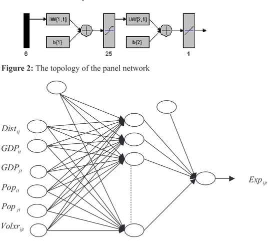
In this study, bilateral export flows will be analyzed through a pan-el modpan-el and a neural network modpan-el. In both modpan-els, exactly the same data set and the same explanatory and dependent variables will be used. Equation 3 will be the base for the panel model as well as the neural net-work model. In panel model, distance, real GDP of the exporting (coun-try i) and importing coun(coun-try (coun(coun-try j), population of the exporting and importing country and the volatility of exchange rates are regressed on bilateral exports to explain the variation in them. On the other hand, the inputs of the neural network are also the same as the explanatory variables of the panel model (distance, real GDP of the exporting (country i) and importing country (country j), population of the exporting and importing country and volatility of exchange rates). Neural network model is pected to learn the relationship between these 6 inputs and bilateral ex-ports (the output) through neurons in each layer. The hidden layer which processes and sends the information received from the input layer to the output layer consists of 25 neurons. The output layer has one output neu-ron namely bilateral exports from country i to country j. The structure of the neural network model is shown in Figure 1 and Figure 2. Our network has tan-sigmoid transfer function in the hidden layer and a linear transfer function in the output layer.
Figure 1: The multilayer network with 6 inputs, 25 hidden neurons and 1 output
Figure 2: The topology of the panel network
7. COMPARISON BETWEEN PANEL DATA ANALYSIS AND NEURAL NETWORK MODEL
7.1 Results of Panel Data Analysis
The data set used in this study consists of bilateral export flows, GDPs, population, volatility of exchange rates and distances among the EU-15 countries from 1964 to 2003. For each country pair we have 40 years of data. To see whether panel unit roots are present in the data, we first con-duct several panel unit root tests and and based on the test results suggest-ed by Levin-Lin-Chu (2002), we conclude that panel unit roots are not systematically present in the data.
Our initial attempt is to investigate how trade flows across European countries can be explained by income, population, distance and also vol-atility of exchange rates. To this aim, we apply panel data analysis on the basis of Equation 3.
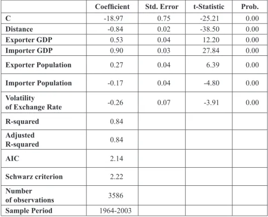
Table 1 shows the results of panel data analysis that are in consistency with the international trade theory. The results indicate that as distance becomes larger, bilateral trade between countries tends to decrease. Fur-thermore, higher income in the exporting country has a positive effect on bilateral trade by leading to more production and higher exports. As Table 1 shows, when income of exporting country increases by 1%, its exports increase by 0.53%. For a very similar reason, higher income tends to in-crease the level of imports as well. According to Table 1, a 1% inin-crease in the importing country’s real GDP increases its imports by 0.90%.
Table 1: Panel least squares with period fixed effects, dependent variable:
log of real bilateral exports
Coefficient Std. Error t-Statistic Prob.
C -18.97 0.75 -25.21 0.00 Distance -0.84 0.02 -38.50 0.00 Exporter GDP 0.53 0.04 12.20 0.00 Importer GDP 0.90 0.03 27.84 0.00 Exporter Population 0.27 0.04 6.39 0.00 Importer Population -0.17 0.04 -4.80 0.00 Volatility of Exchange Rate -0.26 0.07 -3.91 0.00 R-squared 0.84 Adjusted R-squared 0.84 AIC 2.14 Schwarz criterion 2.22 Number of observations 3586 Sample Period 1964-2003
Additionally, population of the exporting country has a positive effect on bilateral exports. This shows that higher population will create opportu-nities for specialization which will boost production and exports from that country. The last variable of interest is the volatility of exchange rates. Our results indicate that volatility of exchange rates has a negative effect on real bilateral exports. For all variables that are used to explain the variance in bilateral exports, coefficients are highly significant.
7.2 Results of the Neural Network Model
This section deals mainly with the feed-forward network used to ana-lyze bilateral exports across European countries and their determinants.
Before constructing and training the network, the inputs (distance, GDP and population of exporting and importing country, volatility of exchange rates) and targets (bilateral exports) are normalized so that the mean is zero and variance unity. In some situations, the input vector has a large dimension, but the correlation among components of the vectors is quite high. In this case, it is useful and necessary to reduce the dimension of in-put vectors. An effective method for performing this operation is principal component analysis (Demuth et al., 2002). When we perform principal components analysis, we see no redundancy in our data set, because the size of input vectors does not reduce.
The objective of model selection is to construct a model with accept-able levels of model bias and variance. Therefore, it is necessary to divide the data set into three subsets: training, validation and test sets. The train-ing set is used to determine the network parameters: weights and biases. Weights show how strongly a signal from one node affects the other node, while bias influences the strength of the effects of inputs on the output. So, the net effect of an explanatory variable or input on the output is calculated as the product of the input and weight, including the impact of the bias. The outcome of the validation set is predicted by using these weights and biases calculated using the examples given in the training set. Then, the network architecture –a combination of weights, biases and the number of hidden neurons- that gives the smallest validation set error is chosen and the network`s performance is evaluated by using the test set (Hung et al., 2002).
The network is trained using early stopping which is a method em-ployed for improving generalization. In this method, while the network is being trained the error on the validation set is observed simultaneously. The training and validation set error normally decreases during the initial stage of training. However, the error on the validation set starts increasing when the network begins to overfit the data. When the validation set error increases for a pre-determined number of iterations, the training must be stopped, and the weights as well as biases which result in minimum vali-dation set error are accepted (Demuth et al., 2002).
After dividing the data set into three subsets, a feedforward network with two layers is created as shown in Figure 1 and 2. The number of neu-rons in the hidden layer is selected experimentally. As stated in the litera-ture, too many hidden layers may cause overfitting of the data resulting in a low model bias and a high model variance. It is found that the network with 25 hidden neurons gives quite satisfactory results.
The Levenberg-Marquardt training function is used to train the network. This is a numerical optimization technique and is especially adapted to the minimization of the error. This algorithm is known as the fastest technique for training moderate-sized feedforward neural networks (Demuth et al., 2002). One advantage of this training method is its fast convergence about minimum and its good prediction performance (Köker, 2007). Kişi (2004) provides a comprehensive explanation for this algorithm.
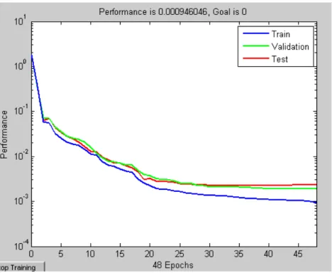
Training results of the network are shown in Figure 3. As the figure shows, when the number of epochs increases the errors of all three sets decline. At the beginning of training, the decrease in squared error is very sharp, but then it decreases at a lesser pace. In our neural network, training is stopped after 48 epochs, because at that point the error for validation set starts increasing. If the model is constructed successfully, the test set and validation set error should show similar characteristics. Figure 3 shows that they both follow the same pattern which proves that our model is re-liable. The performance of the model is measured with the mean squared error which reduces to 0.00095 after 48 epochs.
Figure 3: Training, validation and test set errors
The errors on the training, validation and test sets are the first means to obtain some information about the performance of a trained network. However, the network response needs to be measured in more detail. One choice is to carry out a regression analysis between the network response which are outputs produced by the network and the corresponding targets that are actual outputs in the data set (Demuth et al., 2002).
Therefore, the next step is to simulate the trained network. Since the targets were normalized before constructing the network so that the mean was 0 and the standard deviation was 1, the network outputs are needed to be transformed back into the original units.
In a linear regression analysis between the network outputs and the cor-responding targets, there are two parameters to interpret:
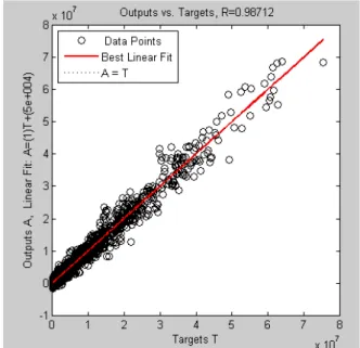
m = 1.0001 r = 0.9871
The first parameter m stands for the slope of the best linear regres-sion between targets (actual outputs) and network outputs. In the case of a perfect fit, which means network outputs exactly equal to the targets, the slope should be 1. The second statistic r is the correlation coefficient (R-value) between network outputs and targets. It shows how well the var-iation in network output is explicated by the targets. If this number is equal to 1, then there is perfect correlation between targets and network outputs (Li and Liu, 2005). In our results, the numbers are very close to 1, which implies a very good fit. To compare neural network model with panel least squares we need R-squared for the neural network model which is the square of the correlation between targets and network outputs (r, R-value). R-squared calculated is 0.97. According to this value of R-squared, it is possible to conclude that the neural network model can explain 97% of the variation in bilateral exports with the given 6 inputs.
In Figure 4, the network outputs are plotted against the targets. The best linear fit is displayed by a dashed line. The perfect fit, which requires network outputs equal to targets, is shown by the solid line. Here, it is very difficult to differentiate the best linear fit line from the perfect fit line be-cause the fit is very good.
7.3. Forecasting Performance of the Neural Network and the Panel Model
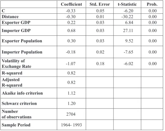
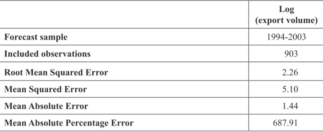
In this section, the performance of the panel model will be compared with that of neural network model in out-of-sample forecasting. To per-form this, a panel least squares model is estimated with period fixed ef-fects using the data from 1964 to 1993 and this model is used to forecast bilateral export volumes from 1994 to 2003. The estimation output and the results of panel model forecasting are shown in Table 2 and 3 respectively. A neural network model calculates MSE based on standardized data, while the panel model errors are based on non-standardized data. To make a fair comparison, the whole dataset is standardized before running the regres-sion and the forecasts are obtained. The results shown in Table 2 and 3 indicate that MSE of the panel model is 5.1.
Table 2: Panel Least Squares Model with Period Fixed Effects,
Dependent Variable: Log of Real Bilateral Exports
Coefficient Std. Error t-Statistic Prob.
C -0.33 0.05 -6.20 0.00 Distance -0.30 0.01 -30.22 0.00 Exporter GDP 0.22 0.03 6.84 0.00 Importer GDP 0.68 0.03 27.11 0.00 Exporter Population 0.30 0.03 9.52 0.00 Importer Population -0.18 0.02 -7.65 0.00 Volatility of Exchange Rate -1.07 0.18 -6.02 0.00 R-squared 0.82 Adjusted R-squared 0.82
Akaike info criterion 1.12
Schwarz criterion 1.20
Number
of observations 2704
Table 3: Forecast Results of Panel Least Squares Model with Period Fixed Effects Log (export volume) Forecast sample 1994-2003 Included observations 903
Root Mean Squared Error 2.26
Mean Squared Error 5.10
Mean Absolute Error 1.44
Mean Absolute Percentage Error 687.91
On the other hand, the data set that will be used in the neural network model is divided into two parts. The first part consists of the years from 1964 to 1993 and is used to construct and train the neural network. The sec-ond part which includes the data from 1994 to 2003 is used to test the con-structed neural network in terms of mean squared error and R-squared, and to make a comparison between neural network and panel data forecasting.
After constructing and training the network, mean squared errors are obtained for the three subsets of the first part of the data set (years from 1964 to 1993). MSE is calculated as the average squared difference be-tween normalized network outputs and targets. Table 4 shows the mean squared error and R-value for training, validation and test sets.
Table 4: Training Results
Number of Samples
(Total: 2683) MSE R-value
Training 1341 1.25697e-3 0.99
Validation 671 1.95853e-3 0.98
Test 671 1.98984e-3 0.98
Since 25% of the whole sample is employed as validation set and the other 25% as test set, 1341 data points out of 2683 are used for training the network. The regression R-value shown in Table 4 measures the
correla-tion between unnormalized network outputs and targets for each subset. It is seen that for each subset we have satisfactorily high R- values.
After constructing the neural network by using the data from 1964 to 1993, we use the rest of the data set, which is from 1994 to 2003, to test the network’s performance. If the network has learned the relationship be-tween inputs and outputs appropriately, it is expected to perform well when a new data set is introduced to it. The performance of a neural network is measured as follows: The network determines the weights and biases us-ing the trainus-ing set chosen from the observation points between the years 1964-1993. Then, the neural network is asked to produce its own outputs that are bilateral export volumes for the years from 1994 to 2003, for giv-en input values for the same period (GDP and population of exporting and importing country, distance and volatility of exchange rates). Then, actual/observed values of bilateral export volumes from 1994 to 2003 are compared with the ones that neural network produces using its predicted weights and biases. MSE is computed by comparing the network`s outputs with observed values of bilateral exports from 1994 to 2003.
When the test set which has 903 observations - from 1994 to 2003- is in-troduced to the neural network, it yields the results summarized in Table 5. Table 5: The Test Results of the Neural Network Model
Number of Samples MSE R-value
Test Set 903 2.11193e-2 0.9176
R-squared for the test set is calculated as the square of the R-value in Table 5 and it is 0.84. A comparison between R-squared produced by neural networks (0.84) and panel model (0.82) reveals that neural network modeling offers slightly higher explanatory power.
When the MSE of neural network model -which is 0.0211- is compared to the MSE produced by panel data forecasting -which is 5.1- it is seen that neural networks offer a much lower MSE. The reason why there is so much difference between neural network and panel model forecasts is that the regression model uses logged data set while inputs given into the neural network are non-logged. Therefore, MSE of panel model is recom-puted for logged data in terms of non-logged data. It is done as follows:
First, forecasts are computed in logs and then are transformed using the exponential into the forecasts of the variable without logs. Lastly, MSE is computed based on these predictions, which is 2.97. Our analysis reveals that there is still a large discrepancy between the MSE produced by the neural network model (0.0211) and panel model (2.97) which suggests that neural networks lead to much better out-of-sample forecasting perfor-mance than the panel model.
8. CONCLUSION
This study compares the results given by panel data analysis and neural networks in analyzing bilateral trade flows. Both models give satisfactory results which show that our modified gravity model of bilateral trade can well explain the variation in bilateral exports among European countries from 1964 to 2003. Balanced panel estimates have the advantage of plaining the individual effect of each independent variable on bilateral ex-ports and showing whether this effect is significant or not. R-squared given by panel data analysis for the period between 1964 - 2003 is 84%, which shows that 84% of the variation in bilateral exports can be explained by distance, GDP and population of exporting and importing countries, and the volatility of exchange rates in our sample. When we construct a neural network by using the same independent and dependent variables, we find that 97% of the variation in bilateral exports can be explained with these variables. Neural networks seem superior to traditional panel data analysis in explaining bilateral exports when R-squared is used as a criterion.
When we make out-of-sample forecasting by employing a panel model with period fixed effects, and use the period that is forecasted in panel model as the test set of the neural network, we see that neural networks produce much lower MSE (0.02) which makes them superior to the panel model with a MSE of 2.97. One of the main relative benefits of the neu-ral network model is nonlinearity, as it uses sigmoid functions instead of linear functions as building blocks. This partly explains its success in our study. Our paper shows that neural networks could be employed in eco-nomics sometimes as an alternative and yet sometimes as a complement to the statistical methods, and may lead to satisfactory results which are in accordance with the international trade literature.
ACKNOWLEDGEMENTS
The author would like to thank to Prof. Dr. Ertuğrul Taçgın from Mar-mara University for giving the idea of combining econometric research with the neural networks; to Prof. Dr. Robert M. Kunst of the University of Vienna for his precious guidance throughout the paper and PhD Disserta-tion, Prof. Dr. Jesus Crespo-Cuaresmo from the Vienna University of Eco-nomics and Business for his helpful comments and friendly supervision.
REFERENCES
ANDERSON J. E., (1979), “A theoretical foundation for the gravity equa-tion”, American Economic Review, Vol. 69, Issue 1, pp.106–116. ANDERSON J., VAN WINCOOP E., (2003), “Gravity with Gravitas: a
solution to the border puzzle”, American Economic Review, Vol. 93, Issue 1, pp.170–192.
BALOGUN, E. D., (2007), Effects of Exchange Rate Policy on Bilateral Export Trade of WAMZ Countries, MPRA Paper, No: 6234.
BALDWIN R., TAGLIONI D., (2006), “Gravity for dummies and dum-mies for gravity equations”, NBER Working Paper, No: 12516. BALTAGI B. H., EGGER P., PFAFFERMAYR M., (2003), “A generalized
design of bilateral trade flow models”, Economics Letters, Vol. 80, pp.391–397.
BERGSTRAND, J. H., (1989), “The Generalized Gravity Equation, Mo-nopolistic Competition, and the Factor-proportions Theory in Interna-tional Trade”, The Review of Economics and Statistics, Vol. 71, Issue 1, pp. 143-153.
CHATFIELD, C., (1993), “Neural networks: Forecasting Breakthrough or Passing Fad?”, International Journal of Forecasting, Vol. 9, pp. 1-3. CHATFIELD, C., (1995), “Positive or Negative? ”, International
CHATFIELD, C., (1997), “Forecasting in the 1990s”. The Statistician, Vol. 46, Issue 4, pp. 461-473.
CHURCH, K. B., and CURRAM S. P., (1996), “Forecasting Consumers’ Expenditure: A Comparison between Econometric and Neural Network Models”, International Journal of Forecasting, Vol. 12, pp. 255-267. CLARK, P., TAMIRISA, N., WEI, S. J., SADIKOV, A., and ZENG, L.,
(2004), “Exchange Rate Volatility and Trade Flows - Some New Evi-dence”. International Monetary Fund.
CUSHMAN, D. O., (1983), “The Effects of Real Exchange Rate Risk on International Trade”, Journal of International Economics, Vol. 15, pp. 45-63.
DE GRAUWE P., and DE BELEFROID B., (1986), “Long Run Exchange Rate Variability and International Trade”. In S. Arndt and J.D. Richard-son (Eds.), Real Financial Linkages Among Open Economies (Chap-ter 8), London: The MIT Press.
DELL`ARICCIA G., (1999), “Exchange Rate Fluctuations and Trade Flows: Evidence from the European Union”. IMF Staff Papers, Vol. 46, Issue 3, pp. 315-334.
DEMUTH, H., BEALE, M., and HAGAN, M., (2002), “Neural Network Toolbox User’s Guide for Use with MATLAB”, Version 4, The Math-works, Natick, MA.
EGGER P., PFAFFERMAYR M., (2003), “The proper panel econometric specification of the gravity equation: a three-way model with bilateral interaction effects”, Empirical Economics, Vol. 28, pp. 571–580. FARAWAY, J., and CHATFIELD, C., (1998), “Time Series Forecasting
with Neural Networks: A Comparative Study Using the Airline Data”,
Applied Statistics, Vol. 47, Issue 2, pp. 231-250.
FRANK, R. H., and BERNANKE, B. S., (2007), Principles of Econom-ics, Mc Graw Hill/Irwin, Boston.
GIOVANIS, E., (2008), “A Panel Data Analysis for the Greenhouse Effects in Fifteen Countries of European Union”, MPRA Paper, No: 10321.
GLICK, R., and ROSE, A. K., (2002), “Does a Currency Union Affect Trade? The Time series Evidence”, European Economic Review, Vol. 46, pp. 1125 – 1151.
GRONHOLDT, L., and MARTENSEN, A., (2005), “Analysing Customer Satisfaction Data: A Comparison of Regression and Artificial Neural Net-works”, International Journal of Market Research, Vol. 47, Issue 2. HARRIS M. N., MATYAS L., (1998), “The econometrics of gravity
mod-els”, Melbourne Institute Working Paper, No: 5/98.
HILL, T., O’CONNOR, M., and REMUS, W., (1996), “Neural Network Models for Time Series Forecasts”, Management Science, Vol. 42, Is-sue 7, pp. 1082-1092.
HORNIK, K., STINCHCOMBE, M., and WHITE, H., (1989), “Multilay-er Feedforward Networks are Univ“Multilay-ersal Approximators”, Neural
Net-works, Vol. 2, pp. 359-368.
HOPTROFF, R.G., (1993), “The Principles and Practice of Time Series Forecasting and Business Modelling Using Neural Nets”, Neural
Computing & Applications, Vol. 1, pp. 59-66.
HORNIK, K., STINCHCOMBE, M., and WHITE, H., (1990), “Univer-sal Approximation of an Unknown Mapping and its Derivatives Using Multilayer Feedforward Networks”, Neural Networks, Vol. 3, Issue 5, pp. 551-560.
HUNG, M. S., SHANKER, M., and HU, M. Y., (2002), “Estimating Breast Cancer Risks Using Neural Networks”, The Journal of the
Opera-tional Research Society, Vol. 53, Issue 2, pp. 222-231.
HUTCHINSON, J. M., LO, W. A., and POGGIO, T., (1994), “A Nonpar-ametric Approach to Pricing and Hedging Derivative Securities via Learning Networks”. The Journal of Finance, Vol. 49, Issue 3, pp. 851-889. Papers and Proceedings Fifty-Fourth Annual Meeting of the American Finance Association: Boston, Massachusetts, January 3-5. KABUNDI, A. N., (2004), “Using Artificial Neural Networks to Forecast
KISI, Ö., (2004), “Multi-layer Perceptrons with Levenberg-Marquardt Training Algorithm for Suspended Sediment Concentration Prediction and Estimation”, Hydrological Sciences–Journal–des Sciences
Hy-drologiques, Vol. 49, Issue 6, pp. 1025-1040.
KOWALSKI, P., (2006), “The Impact of the Economic and Monetary Union in the EU on International Trade- A Reinvestigation of the Exchange Rate Volatility Channel”, PhD Thesis submitted at the Uni-versity of Sussex.
KOKER, R., ALTINKOK, N., and DEMIR, A., (2007), “Neural Network Based Prediction of Mechanical Properties of Particulate Reinforced Metal Matrix Composites Using Various Training Algorithms,
Materi-als and Design, Vol. 28,pp. 616-627.
KUAN, C. M., and LIU, T., (1995), “Forecasting Exchange Rates Using Feedforward and Recurrent Neural Networks”, Journal of Applied
Econometrics, Vol. 10, Issue 4, pp. 347-364.
KUO C., and REITSCH, A., (1995-96), “Neural Networks vs. Convention-al Methods of Forecasting”, JournConvention-al of Business Forecasting
Meth-ods and Systems, Vol. 14, Issue 4, pp. 17-22.
LEVIN, A., LIN C.F. and CHU J., (2002), “Unit root test in panel data: asymptotic and finite sample properties”, Journal of Econometrics, Vol. 108, pp. 1-24.
LI, S., and LIU, Y., (2005), “Parameter Identification Procedure in Groundwater Hydrology Artificial Neural Network”. In D. S. Huang, X. P. Zhang, & G. B. Huang (Eds.), Advances in Intelligent Comput-ing, ICIC Part II, China.
LODEWYCK, R. W., and DENG, P.S., (1993), “Experimentation with a Back-propagation Neural Network, An Application to Planning End User System Development”, Information & Management, Vol. 24, pp. 1-8. MAKRIDAKIS, S., ANDERSON, A., CARBONE, R., FILDES, R.,
HIB-ON, M., LEWANDOWSKI, R., NEWTHIB-ON, J., PARZEN, E., and WIN-KLER, R., (1982), “The Accuracy of Extrapolation (Time Series) Meth-ods: Results of a Forecasting Competition”. Journal of Forecasting, Vol. 1, pp. 111-153.
MATLAB@ Version 7.4.0.287, The MathWorks, Inc. R2007a.
MATYAS, L., (1997), “Proper Econometric Specification of the Gravity Model”, World Economy, Vol. 20, Issue 3, pp. 363-368.
MILERIS, R., BOGUSLAUSKAS, Vytautas, (2011), “Credit Risk Esti-mation Model Development Process: Main Steps and Model Improve-ment”, Inzinerine Ekonomika-Engineering Economics, Vol. 22, Is-sue 2, pp. 126-133.
NUROGLU, E., KUNST R. M., (2014), “Competing specifications of the gravity equation: a three-way model, bilateral interaction effects, or a dynamic gravity model with time varying country effects? ”, Empirical
Economics, Vol. 46, pp. 733–741.
OLIVERIO, M., YOTOV, Y., (2010), “Dynamic gravity: endogenous country size and asset accumulation”, Canadian Journal of
Econom-ics, Vol. 45, Issue 1, pp. 64–92.
ÖZTEMEL, E., (2003), Yapay Sinir Ağları, Papatya Yayıncılık, İstanbul. QI, M., (1999), “Nonlinear Predictability of Stock Returns Using Finan-cial and Economic Variables”, Journal of Business and Economic
Statistics, Vol. 17, Issue 4, pp. 419-429.
REFENES, A. N., AZEMA-BARAC, M., CHEN, L., and KAROUSSOS, S. A., (1993), “Currency Exchange Rate Prediction and Neural Net-work Design Strategies”, Neural Computing and Applications, Vol. 1, pp. 46-58.
ROSE, A. K., LOCKWOOD, B., and QUAH D., (2000), “One Money, One Market: The Effect of Common Currencies on Trade”,. Economic
Policy, Vol. 15, Issue 30, pp. 7-45.
SAKALAS, A., VIRBICKAITE, R., (2011), “Construct of the Model of Crisis Situation Diagnosis in a Company”, Inzinerine
Ekonomi-ka-Engineering Economics, Vol. 22, Issue 3, pp. 255-261.
SHACHMUROVE, Y., (2002), “Applying Artificial Neural Networks to Business, Economics and Finance”, Penn CARESS Working Papers, University of Pennsylvania.
TINBERGEN, J., (1962), Shaping the World Economy: Suggestions for an International Economic Policy, Twentieth Century Fund, New York.
WEST, P. M., BROCKETT, P. L., and GOLDEN, L. L., (1997), “Com-parative Analysis of Neural Networks and Statistical Methods for Pre-dicting Consumer Choice”, Marketing Science, Vol. 16, Issue 4, pp. 370-391.
WHITE, H., (1990), “Connectionist Nonparametric Regression: Multi-layer Feedforward Networks Can Learn Arbitrary Mappings”, Neural