An Approximation Algorithm for Computing the Visibility Region of a
Point on a Terrain and Visibility Testing
Sharareh Alipour
1, Mohammad Ghodsi
2, Ugur Gudukbay
3and Morteza Golkari
11Department of Computer Engineering, Sharif University of Technology, Tehran, Iran 2Department of Computer Engineering,
Sharif University of Technology and Institute for Research in Fundamental Sciences (IPM), Tehran, Iran∗ 3Department of Computer Engineering, Bilkent University, Ankara, Turkey
[email protected], [email protected], [email protected], [email protected]
Keywords: Computational Geometry, Visibility, Approximation Algorithm, Terrain.
Abstract: Given a terrain and a query point p on or above it, we want to count the number of triangles of terrain that are visible from p. We present an approximation algorithm to solve this problem. We implement the algorithm and then we run it on the real data sets. The experimental results show that our approximation solution is very close to the real solution and compare to the other similar works, the running time of our algorithm is better than their algorithm. The analysis of time complexity of algorithm is also presented. Also, we consider visibility testing problem, where the goal is to test whether p and a given triangle of train are visible or not. We propose an algorithm for this problem and show that the average running time of this algorithm will be the same as running time of the case where we want to test the visibility between two query point p and q.
1
INTRODUCTION
Problem Statement. Suppose that T is a set of n disjoint triangles representing a terrain. Two points p, q ∈ R3 are visible to each other with respect to
(w.r.t.) T if the line segment pq does not intersect any triangle of T . A triangle ∆ ∈ T is also considered to be visible (w.r.t. T ) from a point p if there exists a point q ∈ ∆ such that p and q are visible to each other. Here, the visibility counting problem (VCP) is to find the number of triangles of T which are visible from any query point p. The visibility testing prob-lem (VTP) is also defined as follows: given a query point p and a triangle ∆ ∈ T we want to test whether pand ∆ are visible or not.
Definition 1.1. The set of all points that are visible from a query point p is the visibility region of p de-noted by V R(p).
Related Work. Computing the visible region of a point is a well-known problem appearing in numerous applications (see, e.g., (Cohen-Or and Shaked, 1995; Cole and Sharir, 1989; Floriani and Magillo, 1994; Floriani and Magillo, 1996; Franklin et al., 1994; Goodchild and Lee, 1989; Stewart, 1998)). For ex-∗This research was in part supported by a grant from IPM. (No. CS1390-2-01)
ample, the coverage area of an antenna for which line of sight is required may be approximated by clipping the region that is visible from the tip of the antenna with an appropriate disk centered at the antenna. As a similar problem, natural resource extractors may wish to site visual nuisances, such as clearcut forests and open-pit mines, where they cannot be seen from pub-lic roads. Also, zoning laws in some regions, such as the Adirondack Park of New York State, may pro-hibit new buildings that can be seen from a public lake (Franklin et al., 1994).
The complexity of computing the visibility region of a point, VR(p), might be Ω(n2) (Cole and Sharir, 1989; Devai, 1986), where n is the number of trian-gles in T . Therefore, approximation algorithms which compute an approximation of VR(p) can highly re-duce the running time.
Moreover, a good approximation of the visible re-gion is often sufficient, especially when the triangula-tion itself is only a rough approximatriangula-tion of the under-lying terrain (Ben-Moshe et al., 2008). Note that the terrain representation is fixed and cannot be modified during the running time of the algorithm.
In (Ben-Moshe et al., 2008) a generic radar-like algorithm is presented for computing an approxima-tion of V R(p). The algorithm extrapolates the visi-ble region between two consecutive rays (emanating
from p) whenever the rays are close enough; that is, whenever the difference between the sets of visible segments along the cross sections in the directions specified by the rays is below some threshold. Thus, the density of the sampling by rays is sensitive to the shape of the visible region. Ben-Moshe et al. sug-gest a specific way to measure the resemblance (dif-ference) and to extrapolate the visible region between two consecutive rays. They also present an alterna-tive algorithm which uses circles of increasing radii centered at p instead of rays emanating from p. Both algorithms compute a representation of the (approx-imated) visible region that is especially suitable for visibility from p queries.
Overall they used four algorithms, Fixed ECH, ECH, Fixed radar-like and Radar-like to approximate V R(p). It is shown that Radar-like algorithm is the fastest among these four algorithms.
Our Result. We present an algorithm to approx-imate the number of visible triangles from a query point p which is noted by mp. Moreover, the
algo-rithm can be used to approximate V R(p). We also consider the visibility testing problem and present our experimental results. The structure of the paper is as follows: in section 2, we present the algorithm for visibility testing problem and then we implement the algorithm on real data sets. We show that the aver-age running time of this algorithm for VTP between a point and a triangle is O( f (n)) in which f (n) is the running time of VTP for two points. In section 3, we present the approximation algorithm for the visibility counting problem and also an exact algorithm which is used to compare the approximated solution to the exact solution. In section 4, we provide the experi-mental results of the proposed algorithm. We com-pare our results to the results of (Ben-Moshe et al., 2008).
2
VISIBILITY TESTING
PROBLEM
Suppose that we are given a set S of n triangles in R3 and a query point p. We classify the visible triangles of S from p into two groups:
• A triangle is an edge-visible triangle if there is a point on its edges that is visible from p.
• If the triangle is visible from p but there is not any visible point on its edges, then it is called a mid-visible triangle.
Lemma 2.1. If the triangles of S form a terrain, then all the visible triangles from a query point p are edge-visible.
Using Lemma 2.1, to compute the number of vis-ible triangles of a terrain from a given query point p, it is enough to consider the edges of triangles.
2.1
The Proposed Algorithm for VTP
According to Lemma 2.1, if a triangle ∆1∈ T is
visi-ble to a query point p, then ∆1is edge-visible.
There-fore, for each edge of ∆1, begin from one of its
ver-tices, such as a1 . If a1and p are visible, then ∆1
is visible to p and we break the algorithm, else we choose the first triangle ∆2hit by the ray emanating
from p to a1. ∆2covers some part of that edge. So,
it is enough to check whether the remained part of the edge is visible to p. For the remained part, we con-sider the first point a2on that edge which is not
cov-ered by ∆2. We shoot a ray from a2to p. If a2and p
are visible then ∆1and p are visible, else we consider
the first triangle hit by the ray emanating from a2to
p. The same as ∆1, we run the algorithm on ∆2. If we
reach the end of edge, then that edge is not visible to p. If all the three edges of ∆1are invisible to p then
∆1is also invisible to p (See Algorithm 1).
Algorithm 1:Algorithm for VTP.
Input: ∆ ∈ T .
p: a query point Output:
A boolean indicates whether triangle ∆ is visible to p or not.
Method:
1: Create three line segments s1,s2and s3based on
∆’s edges.
2: Initialize segments queue segQueue with s1,s2
and s3.
3: while segQueue is not empty do
4: seg = segQueue.pop()
5: if At least one point on the line segment seg is visible from p then
6: return true
7: else
8: Find the first concealer triangle TCfor
invis-ible point p on the line segment seg.
9: for each segment segt of segments queue
segQueue do
10: COVER LINE SEGMENT(p,TC, segt)
11: end for
12: end if
13: end while
2.2
Experimental Results of VTP
According to the Algorithm 1, the running time of Al-gorithm 1 for each query point p and triangle ∆1
de-pends on the number of ray shootings which is equal to the number of triangles covering the edges of ∆1.
We denote this number by tp(∆1). Therefore, the
run-ning time of this algorithm is O(tp(∆) f (n)) in which
f(n) is the time for each ray shooting. In our data sets each the terrain is represented as a height field that for each point (i, j) on the regular 2D grid, a height value is specified. The regular grid is triangulated to represent the terrain. We use a regular triangula-tion such that for every four points x1= (i, j, k1), x2=
(i + 1, j, k2), x3= (i, j + 1, k3), x4= (i + 1, j + 1, k4),
two triangles are constructed: ∆1= (x1, x2, x4) and
∆2= (x1, x3, x4). In our expriments we do not
pre-process the triangles of terrain, so f (n) = O(p(n)). In each of the data sets, we choose random points and run Algorithm 1 for each point p and each of the tri-angles of the terrain. For each triangle ∆1∈ T , we
calculate tp(∆1). The experimental results indicate:
E(tp(∆1)) = ∑n∆i∈Ttp(∆i)/n = O(1)
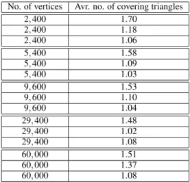
which means that the average number of triangles covering a triangle for a random query point is O(1). So, the average running time of visibility testing be-tween a triangle and a random query point is O( f (n)). In Table 1 the average of tpis mentioned for each data
set which is not greater than 2 in none of them. It is shown that the average number of tp(∆) is
indepen-dent of the size of data set.
Table 1: The average number of triangles that cover a trian-gle according to a random query point for each data set.
No. of vertices Avr. no. of covering triangles 2, 400 1.70 2, 400 1.18 2, 400 1.06 5, 400 1.58 5, 400 1.09 5, 400 1.03 9, 600 1.53 9, 600 1.10 9, 600 1.04 29, 400 1.48 29, 400 1.02 29, 400 1.08 60, 000 1.51 60, 000 1.37 60, 000 1.08
3
THE VISIBILITY COUNTING
PROBLEM
Our visibility counting algorithm is based on count-ing the number of triangles whose vertices are visi-ble from the query point. So, to compute the visivisi-ble region of a query point p, we compute the triangles whose vertices are visible from p.
3.1
Approximation Algorithm for VCP
For each query point p, if at least one of the vertices of a triangle is visible to p, then we consider it as a visible triangle. To compute the number of triangles which at least one of their vertices are visible to p, we propose the following algorithm:
First, we select the triangle ∆1that is intersected
by the ray emanating from p to the surface of T . Ob-viously ∆1is visible to p. In the next step, we
con-sider the three neighbors of ∆1; we check whether
the vertices of these triangles are visible to p. If at least one of the vertices of these triangles is visible to p, then the triangle is visible to p. We run the al-gorithm recursively on the neighbors of the triangles. Otherwise, we decide that the triangle is an invisible triangle. For each non-visible triangle, we shoot a ray emanating from p to the vertices of visible triangles; the first triangle hit by that ray is considered as a vis-ible triangle and we recursively run the algorithm on its neighbors. Algorithm 2 shows pseudo code of this algorithm.
3.2
Time Complexity
In Algorithm 2 each triangle is entered to the queue just once and for each triangle we shoot three rays to the vertices of that triangle. In each step of ray shoot-ing, we check whether there is a triangle between p and a vertex or we want to find the first triangle hit by a ray emanating from p to a specific direction. In both of these ray shootings, we have to check at most O(√n) triangles. So, the running time of the algo-rithm is O(√nmp) ( where mpis the number of
vis-ible triangles). Note that if we preprocess the trian-gles, each ray shooting takes O(log n) time and this reduces the running time. In our algorithm, we do not preprocess the triangles.
3.3
Exact Algorithm for VCP
Using Algorithm 1, we test whether each triangle of T is visible to p. So, we can compute the exact number of visible triangles. The running time of this algo-rithm is not important and we only use it in our
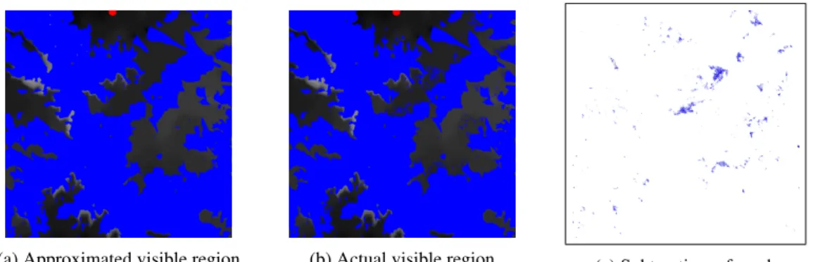
exper-(a) Approximated visible region (b) Actual visible region (c) Subtraction a from b
Figure 1: The approximate (a) and the exact (b) visible region of the query point p(3.3, 242.5, 2089.5). The query point shown in red.
(a) Approximated visible region (b) Actual visible region (c) Subtraction a from b
Figure 2: The approximate (a) and the exact (b) visible region of the query point p(468.8, 232.5, 3228.6). The query point shown in red.
imental result to show that the approximate number of visible triangles is close to the exact number of visible triangles.
4
EXPERIMENTAL RESULTS OF
VCP
We ran the approximation algorithm on three real ter-rain data sets. As it is said, the terter-rain is represented as a height field that for each point (i, j) on the reg-ular 2D grid, a height value is specified. The regreg-ular grid is triangulated to represent the terrain. We use a regular triangulation such that for every four points x1= (i, j, k1), x2= (i + 1, j, k2), x3= (i, j + 1, k3), x4=
(i + 1, j + 1, k4), two triangles are constructed: ∆1=
(x1, x2, x4) and ∆2= (x1, x3, x4). Then, we run the
pro-posed algorithm on height-field representation of the terrain.
Figures 1 and 2 show the actual and approximate visible regions of two query points. We calculate the approximate visible region of a query point using Al-gorithm 2 and use the exact alAl-gorithm to calculate the exact number of visible region of a query point. It is seen that the approximated visibility region of a
query point is close to the actual visibility region of that point.
We define the following error measure. Let m0pbe the number of approximated visible triangles. Then the error associated with m0p is (mp− m0p) divided
by mp. For each data set, we choose 1000 random
query points and for each query point p, we calcu-late the value of mpand m0pand then the error of the
algorithm. Each random point is chosen in different heights above the terrain. It is obvious that the in-crease in the height of a point results in the inin-crease of the number of visible triangles and the running time as well. In Table 2 the average time and average error are mentioned for each data set.
We compare our results to the results of the ap-proach proposed by Ben-Moshe et al. (Ben-Moshe et al., 2008). They proposed four algorithms and mea-sured the performances of these algorithms. We use data sets similar to the ones used in the experiments presented in (Ben-Moshe et al., 2008). In their ex-periment, they have considered ten input terrains rep-resenting ten different and varied geographic regions. Each input terrain covers a rectangular area of approx-imately 5000 − 10000 triangle vertices. For each ter-rain, they picked several view points (x, y coordinates)
Table 2: The average running time for each data set. For each data set, the height of some random points are chosen as specific values.
No. of vertices Running time (ms) Error (%) 2, 400 17 1.39 2, 400 14 0.45 2, 400 13 0.41 5, 400 44 2.03 5, 400 36 0.89 5, 400 28 0.45 9, 600 90 2.28 9, 600 80 1.17 9, 600 66 0.90 29, 400 355 3.92 29, 400 396 1.78 29, 400 365 2.47 60, 000 840 5.28 60, 000 870 3.17 60, 000 954 3.70
Algorithm 2:Approximation algorithm for computing the visible triangles.
Input:
T: A 2D array of triangles. e: A query point p. Output:
The number of visible segments from p. Method:
1: Create empty Queue, bfsQueue.
2: Find triangle ∆1that is intersected by the ray
em-anating from p to the surface of terrain.
3: Add ∆1to bfsQueue.
4: while bfsQueue is not empty do
5: ∆t= bfsQuere.pop()
6: if At least one vertex of triangle ∆t is visible
from p then
7: Add three neighbors of ∆1to bfsQueue.
8: else
9: Find first triangles cover vertices of triangle ∆t.
10: Shoot rays from p to the vertices of these triangles
11: Find hit points of shooting ray and surface of terrain.
12: Add triangles corresponding to the hit points, to bfsQueue.
13: end if
14: end while
nates) randomly. For each query point p, they ap-plied each of the four approximation algorithms (as well as the exact algorithm) 20 times: once for each combination of height (either 1, 10, 20, or 50 meters above the surface of T) and range of sight (either 500,
1000, 1500, 2500, or 3500 meters). For each (approx-imated) region that was obtained, they computed the associated error, according to their defined error mea-sure.
Their defined error measure is as follows: Let Rp
be an approximation of Rpobtained by some
approxi-mation algorithm, where Rpis the region visible from
p. Then the error associated with Rp is the area of
the XOR of Rp and R0p, divided by the area of the
sight that is in use. Note that in the case that Rpis
little in compare with the sight and the difference be-tween R0pand Rpis big in compare with Rp, then the
error will be very little. However, the difference be-tween R0pand Rpis so big. Thus, our error measure
is more accurate than theirs. Each data set in their al-gorithm contains 5000 − 10000 triangle vertices. We also choose some data sets such that the number of triangles in each set is about 10000.
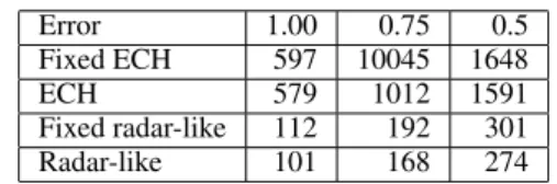
As it is shown in Table 3, the best average running time of their algorithm is 274 ms with the error of 0.5 (using their error measure) whereas the average running time of our proposed algorithm is 70 ms with the error of 0.55 (using our error measure). If we use their error measure, then our error will be 0.35.
Table 3: The results of (Ben-Moshe et al., 2008). They define an error function for approximating the visible region of a query point. According to each error value the running time of their algorithms are mentioned. The best running time is related to Radar-like algorithm.
Error 1.00 0.75 0.5 Fixed ECH 597 10045 1648 ECH 579 1012 1591 Fixed radar-like 112 192 301 Radar-like 101 168 274
The test environment for our experiment and the one used in (Ben-Moshe et al., 2008) are mentioned in Table 4.
Table 4: The properties of platforms of (Ben-Moshe et al., 2008) and ours.
Ben-Moshe Pentium 4 2.4GHz Linux 8.1 Java 1.4 Our platform Pentium 4 2.8GHz Win8 Java 1.7
5
CONCLUSIONS
We propose algorithms for the visibility counting and testing problems on a terrain. We implement our algo-rithm for VTP. Our experimental results shows that in our algorithm, the average running time of visibility testing between a query point and a triangle is almost equal to the running time of visibility testing between two points.
We also proposed an approximation algorithm for VCP and implemented it on real data sets. Our exper-imental results were presented. To compare our al-gorithm with the other related works, we considered the results of (Ben-Moshe et al., 2008), which was a similar work. We showed that in almost similar con-ditions (considering the platforms, the number of tri-angles of terrains) the running time of our algorithm is better than their algorithm. In these algorithms we did not preprocess the data sets. If we preprocess the data sets, the running time of algorithms in the query phase will significantly decrease. Also, we would like to propose exact algorithms for VCP. We are currently extending the proposed algorithms to the case where triangles are in 3D.
REFERENCES
Ben-Moshe, B., Carmi, P., and Katz, M. J. (2008). Ap-proximating the visible region of a point on a terrain. Geoinformatica, 12(1):21–36.
Cohen-Or, D. and Shaked, A. (1995). Visibility and dead-zones in digital terrain maps. Comput. Graph. Forum, 14(3):171–180.
Cole, R. and Sharir, M. (1989). Visibility problems for polyhedral terrains. Journal of Symbolic Computa-tion, 7(1):11 – 30.
Devai, F. (1986). Quadratic bounds for hidden line elim-ination. In Proceedings of the second annual sym-posium on Computational geometry, SCG ’86, pages 269–275, New York, NY, USA. ACM.
Floriani, L. D. and Magillo, P. (1994). Visibility algorithms on triangulated digital terrain models. International journal of geographical information systems, 8(1):13– 41.
Floriani, L. D. and Magillo, P. (1996). Representing the visibility structure of a polyhedral terrain through a horizon map. International journal of geographical information systems, 10(5):541–561.
Franklin, W. R., Ray, C. K., and Shashank, M. (1994). Geo-metric algorithms for siting of air defense missile bat-teries. Battelle Inc., Columbus OH.
Goodchild, M. and Lee, J. (1989). Coverage problems and visibility regions on topographic surfaces. Annals of Operations Research, 18(1):175–186.
Stewart, A. (1998). Fast horizon computation at all points of a terrain with visibility and shading applications. Visualization and Computer Graphics, IEEE Transac-tions on, 4(1):82–93.