Applying Deep Learning in Augmented Reality Tracking
Omer Akgul
∗Bilkent University
Department of Computer Engineering
[email protected]
H. Ibrahim Penekli
Cadem Vision
[email protected]
Yakup Genc
Gebze Technical University
Department of Computer Engineering
[email protected]
Abstract
An existing deep learning architecture has been adapted to solve the detection problem in camera-based tracking for augmented reality (AR). A known target, in this case a planar object, is rendered under various viewing conditions including varying orientation, scale, illumination and sensor noise. The resulting corpus is used to train a convolutional neural network to match given patches in an incoming image. The results show comparable or better performance compared to state of art methods. Timing performance of the detector needs improvement but when considered in conjunction with the robust pose estimation process promising results are shown.
1. Introduction
As a man-machine interface technology, AR (Aug-mented Reality) simply renders virtual information on to real objects [1]. In order to achieve geometrically valid rendering, one needs to track the object of interest to be augmented. This can in principle be done using computer vision techniques. The target object of inter-est can be detected and tracked in a live video stream. The target can be a simple planar marker [2, 3] or any three-dimensional (3D) object [4, 5]. Known model of the object can be used to determine the position and
ori-∗Visiting Gebze Technical University
entation of the object. Rendering of the virtual object follows easily.
In practice, two-dimensional (2D) planar targets are frequently used as an object of interest (see Fig-ure 1). These type of targets are easy to track. Many algorithms have been proposed [6, 2, 7] that detect the target in the given image and track it in the consecutive images. Detection algorithms employ a feature-based approach where interest points are matched with that of the reference views.
Figure 1: An example target used frequently in AR applica-tions (target is provided as part of Vuforia SDK)
Recent advances in hardware and algorithms have sparked an interest in deep learning algorithms. Deep learning methods have successfully been used in com-plex recognition tasks such as written digits recognition and object classification. Specifically, convolutional
2016 12th International Conference on Signal-Image Technology & Internet-Based Systems 2016 12th International Conference on Signal-Image Technology & Internet-Based Systems
neural networks (CNNs) have been successfully used in large scale detection tasks [8, 9].
Robust detection of objects for AR is still a chal-lenging problem. As the AR applications are moving more on the mobile devices, efficient and robust detec-tion algorithms are being sought. Since deep learning has shown successful results in large scale object detec-tion, interest point detection can be done using CNNs as well. This paper introduces a study where existing deep learning architectures (e.g., AlexNet and GoogleNet) have been modified to address the target detection prob-lem for AR. We have shown that the resulting detector’s performance is as good as the state of detection algo-rithms and sometimes much better. The method is cur-rently not fast enough to run on mobile devices but work is underway to make it faster.
In the rest of this document, we first review the state of art detection methods for AR tracking. We than introduce our method along with a few others for com-parison. After presenting the experimental results and discussions we conclude with direction for future re-search.
2. Background
Model-based (or target image) AR tracking in-volves two major steps. First, the target is detected in the incoming video stream using a detection algorithm (see [2] for a complete treatment of AR tracking prob-lem). The detection step, also known as tracker initial-ization, yields the pose of the camera with respect to the known target. This initial pose is in turn used by a tracking algorithm in the second step. The tracking continues till the target is no longer tracked in which case the detector step kicks in. Usually tracking is more robust and less time and resource consuming than detec-tion. Therefore, as long as possible, tracking algorithm is employed and detection algorithm is only used when necessary.
Since tracking is out of scope of this paper, the reader is referred to [2] or [5] for further reading. The detection step on the other hand involves finding a set of matches between the incoming and the reference im-ages. Figure 2 depicts the major steps in the detection process. An off-line stage, i.e., training, is employed to find out the most relevant interest point and their iden-tifying descriptors.
Commonly used interest points include [10, 11, 12]. Many descriptors such as SIFT [13], ORB [14] and HIPS [7] exist. These are based on the fact that there are textual information around the interest point that makes the point valuable in matching. The train-ing step concludes by decidtrain-ing what features to use.
Figure 2: The steps of detection in an AR tracking scneario.
During detection step the incoming image goes through the same interest point extraction and feature descriptor calculation processes as in training. The calculated fea-tures are matched against the reference. A model fitting procedure is followed. Usualy robust methods such as RANSAC [15] or one of its variants like PROSAC [16] are employed. The robust fitting procedure ensures that the matched features generate a geometricall consistent model. In particular, for the 2D case, the model is a simple homography [17].
The detection procedure is well established and current work is focused either on improving the ro-bustness of the matching algorithms or speeding up the model fitting procedure. For matching, new feature de-scriptors are being developed that is faster (with a lot of consideration given to mobile devices) [7] and more ro-bust with respect to illumination and pose changes. The model fitting procedure is still one of the bottlenecks in the process as it requires a good ratio of inliers vs out-liers.
The detection step can in principle be done with any detector including a deep neural network based method. Up to our knowledge, there are no work that uses CNNs for detection in AR. Deep learning has been used in object class detection successfully. More re-cent approaches have been successfully used in large scale object detection problems [8, 9]. Platforms such as CAFFE [18] and DIGITS make it possible to eas-ily train new CNNs on powerfull GPUs such as NVidia Tesla K20Xm.
3. The Method
We introduce a deep convolutional neural network detector called DeepAR. It is based on one of the well known CNN architectures, i.e., AlexNet [19]. We also describe an efficient matching algorithm, HIPS [7], that we have implemented for comparison purposes.
DeepAR: Following the feature-based detection approaches, our method treats the correspondence prob-lem as a recognition probprob-lem. A set of keypoints (a.k.a.
interest points or corners) are extracted in the reference image using one of the well-known corner detection al-gorithms such as FAST [11] or Harris [10]. Patches of size 15× 15 pixels are extracted around these key points. In order to learn their representations, we gener-ate a number of rendered views of the target simulating scale, orientation and illumination changes likely to ap-pear in the test images. The patches around the keypoint represents a class. Our problem then becomes a classi-fication task where a given patch is labeled as one of the existing keypoints (see Figure 3).
Figure 3: DeepAR is a CNN-based detector. The detector first extracts a set keypoints. A patch of size 15× 15 pixels is exyracted and fed into to the CNN detector. The patch is classified as one of the n predifined keypoints.
For CNN implementation, we have started with AlexNet [19] and trained our network to detect the patches. Our subsequent tests suggested some minor modifications to the network but for the sake of clarity we have kept the original network as is. We used 100 epochs in training. For training, we used mini batches of size 50. For learning rate an exponential decay func-tion is used. We trained the network using 80% of our data for training and 20% of it for validation. Testing is donee using the test images not present in the training set. We have experimented a few of these parameters and found no significant difference in performance.
HIPS: We have implementend the method de-scribed in [7]. We build feature descriptors from a large set of training images covering the entire range of view-points to achieve a rotation and scale invariant descrip-tor. For each viewpoint, small rotation, transformation and blur is added for increased robustness.
As in the DeepAR case, FAST feature detector is used to detect features on a reference image. 15× 15 patches are extracted around each feature. They are nor-malized such that they have zero mean and unit stan-dard deviation to provide robustness against illumina-tion changes. HIPS requires a 8× 8 sparsely sampled patch extracted from the original patches (see Figure 4). Once the 8× 8 patches has been extracted for all viewpoints, each pixel in the patch is quantised into 5 histogram bins. Each bin represents probability of in-tensity appearance at selected position in all samples around corresponding feature detected. We set the bit
Figure 4: Blue (dark) squares: The sparse 8×8 sampling grid to form a patch. Pink squares with X: The 13 samples selected to form the patch index (better viewed in color).
at selected position of the selected histogram bin, if the intensity appearance probability in the histogram is less than 5%. Otherwise, we clear the bit in the correspond-ing bin on traincorrespond-ing patches (see Figure 5). We set the bit at selected histogram bin if intensity falls into this bin; otherwise, clear the bit on the runtime patches. Thus, fi-nal feature descriptor needs 320 bit (40 bytes) memory for each feature.
Figure 5: Creating histogram bins for a pixel on training.
To match training and runtime descriptors, we need to calculate dissimilarity scores. Dissimilarity scores can be simply computed by counting the number of bits where both bits in the same position equal to ”1”. We simply AND each of descriptor rows and OR the final results. Computing the dissimilarity score requires 5 ANDs, 4 ORs and a bit count of a 64 bit integer. Bit count is computed quickly using lookup tables or a sin-gle CPU instruction if available. We declare a match if dissimilarity score is less than a threshold (typically 5). An indexing scheme is used to avoid linear search when matching with a large database of features. Each of the samples selected (see Figure 4) for the index is
quantized to a single bit: 1 if the intensity is above the mean of the sample and 0 otherwise. The 13 samples are then concatenated to form a 13-bit integer. Only patches with the same index is matched exhaustively.
4. Experimental Verification
The proposed algorithm has been implemented, tested and compared against state of art methods using real data. Two image targets (Pebbles and Pottery) have been used to do the assessments. The reference images of the targets in Figure 6 have been used to train the de-tection algorithms. Five test images per target are used in testing. The test images are given in Figure 7 to pro-vide the reader with an idea about the variation in view-point and imaging conditions compared to the reference targets.
Figure 6: 2D image targets used in the experiments. Peb-bles (left): A well-known target provided by Vuforia . Pottery (right): A custom-made target used in some of our projects.
Figure 7: Test images of the 2D targets used in the experi-ments showing variety in viewpoint and illumination condi-tions.
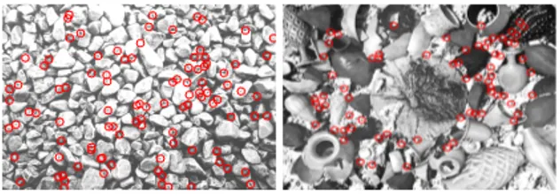
In order to train the algorithms, about 100 cor-ner points are selected using the algorithm described in [11]. These points are shown in Figure 8 overlaid on the reference images. Around 6000 images are ren-dered from the reference view to account for variations in scale, viewing angle, illumination and sensor noise. The rendering process largely follows [7] (see Figure 9 for a few sample patches generated using this process). We have implemented a version of the algorithm by [7] that is fine tuned for best performance on each of the test cases. The algorithm is described in the previous sec-tion for completeness. Some of the details of these fine tuning is outside the scope of this paper. It should be stated for completeness that the implementation shows
better performance than what is reported in the original paper.
Figure 8: The corners used to train for detection (best viewed in color).
Figure 9: A few sample 15× 15 patches extracted around the selected corners for the Pottery marker.
The extracted patches are fed to the training algo-rithm for both DeepAR and HIPS methods. The de-tails of these two algorithms are provided in the pre-vious section. We report the performance of the two algorithms in several different ways. Each provides a particular way of evaluating the results of a detector to be used in an AR tracker.
In order to assess the accuracy of the methods, the test images are manually marked. In other words, the ground truth locations of the markers are known up to sub-pixel accuracy. The manual marking is used to cal-culate the ground truth homography (please see [17] for a detailed discussion on how to calculate the homog-raphy) between the original target and the test image. The accuracy of the estimated homography can be cal-culated using the re-projection error:
εp= ||pm− Hpr||2 (1)
where H is the homography between the reference and the test image, pr is an interest point in the reference
image and pm is the corresponding ground truth
loca-tion of that point.|| · ||2indicates the Euclidean distance calculated with the first two entries of the normalized homogenous coordinates of pm and Hpr, the projected
point in the manually marked test image.
Overall Detector Performance: As explained ear-lier, after the interest points are matched, they are fed to a robust model fitting algorithm, e.g., RANSAC [15], to enforce the geometric constraints leading the pose of the camera. In our case the targets are planar, therefore the geometric constraints will be captured by a 3× 3 homography matrix.
The performance of the final camera pose can be measured using the average re-projection error over all interest points. Table 1 shows the error for estimated homographies for DeepAR and ORB methods. ORB [14] is another detection method that has a commonly used implementation in OpenCV [20]. As expected, DeepAR performs better than ORB as the implemen-tation is optimized for this type of detection tasks.
DeepAR ORB pebble 1 0.852 1.542 pebble 2 3.245 1.163 pebble 3 0.866 4.327 pottery 1 0.821 0.754 pottery 2 52.087 53.978 pottery 3 0.992 54.389
Table 1: Overall performance of the DeepAR compared to ORB. Re-projection error for the calculated homography against the ground truth is calculated using (1).
Interest Point Location: Feature detection is ex-pected to be location sensitive. In other words, if the corners are not located properly, the detectors may not match the right patches in the reference view. Even though the corner detectors (i.e., [10, 11]) are sub-pixel accurate, they tend to generate a lot of superfluous cor-ners. Non-maximal suppression [21] is usually em-ployed to get rid of the extraneous points but it still can cause localization errors. A detector should be immune to patch localization to ease the burden on the robust model fitting procedures such as RANSAC.
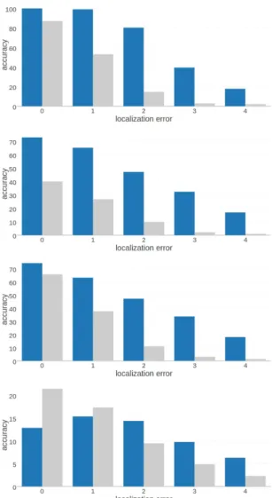
We have tested the detection accuracy when the patch locations are erroneous. For this we have ex-tracted patches within the several pixel neighborhood of the original patch and checked if the match can be estab-lished. Figure 10 shows the result of this test. DeepAR method does very well within close proximity of the original feature except in one of the frames where the viewing angle is quite oblique. It performs consistently better when the distance to the original feature is rela-tively big. This shows that DeepAR method is a detec-tor that can generalize for the cases where the feature localization is poor.
Inliers and Outliers: We would like to make sure that RANSAC process starts with many inliers and at the same time with very little outliers. Figure 11 shows the comparison on number of inliers for both meth-ods. DeepAR method produces consistently more in-liers than HIPS. However, as can be seen in Figure 12 the percentage of inliers vs outliers are less for DeepAR. It generates more inliers but at the same time more out-liers as well. HIPS assigns an uncertainty to the result-ing matches. This is used to filter out most of the
out-Figure 10: Detection accuracy vs feature location error. The ground truth corners in Pottery test images are moved ran-domly within 4 pixel radius. The accuracy of detection is dis-played against the error in the patch location (DeepAR results are shown in dark blue and HIPS results are shown in light gray).
liers. DeepAR finds the close matches with very high certainty. When we look at the rank 2 matches as well, the number of outliers reduces to a quarter. This sug-gests that there are multiple patches with similar signa-tures and a further filtering may be necessary to distin-guish them.
Number of RANSAC Iterations: Another im-plication of having a higher inlier-outlier ratio is that RANSAC may need a high nunber of iterations for finding the homography. In order to test the effect of DeepAR generating higher number of outliers, we de-signed a simple test. For all available test images, we have taken one at random and taken a fixed number (50 matches in this casse) of matches at random. We then
Figure 11: Comparison of number of inliers (i.e., the correct matches) for DeepAR (dark blue) and HIPS (light gray) meth-ods for the Pottery test .
Figure 12: The percentage of inliers against the outliers. RANSAC would prefer a higher number for accuracy and speed. DeepAR (in dark blue) generates more inliers but also a lot of outliers whereas HIPS (in light gray) generates fewer inliers and even fewer outliers.
fed these into RANSAC to find the homography. We calculated the resulting modeling error as explained ear-lier.
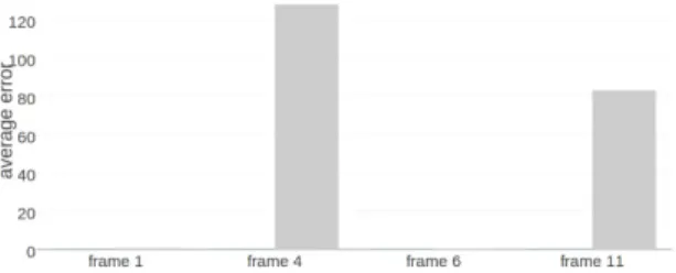
As it can be seen in Figure 13, DeepAR method consistently finds better matches for RANSAC. With a fixed number of iterations, matches provided by DeepAR results in more accurate model fitting. Fig-ure 14 shows the same analysis on individual frames of the Pottery test images. In this case only 200 iterations of RANSAC is used.
Figure 13: The effect of the number of RANSAC itera-tions on accuracy of estimated homography given the detected matches using DeepAR (in dark blue) and HIPS (light gray). Even though DeepAR has larger outlier-inlier ratio, its de-tected features consistently finds better homographies with the same number of RANSAC iterations.
Timing Analysis: An important criterion for
com-Figure 14: For 200 iterations of RANSAC procedure, DeepAR (in dark blue) generates better homographies for all the of the Pottery test images. The results for HIPS is shown in light gray.
paring the detection methods is the timing perfor-mance. DeepAR method works on a given image of size 640x480 pixels in about 3 seconds on an off-the-shelf desktop Nvidia GPU. The detection process for HIPS on the other hand requires on the order tens of mil-liseconds. As explained in the previous paragraphs, the number of iterations required for RANSAC is much less in the case of DeepAR. For similar accuracies, HIPS would need many more number of iterations which could prove to be costly. We cannot make a definitive statement about the benefit of this result yet. Although the time performance of the DeepAR system is not ex-cellent we have observed the potential to make it much faster. The software developed in order to test these models were mostly written in interpreted languages. This significantly dropped our performance. The use of a low level compiled language would be to our bene-fit. Graphical processors on mobile devices has also de-veloped significantly throughout the years. Using these mobile graphical processors will also increase our com-putational speed. However we did not have the time nor resources at the time of writing this paper to experiment with these ideas. Our future work will address this point further.
This section mostly presented the results on the Pottery test images. It should be noted that similar results are observed when the Pebbles test images are used. These are omitted in the text due to space limita-tions.
5. Conclusions
This study has shown that deep convolutional neu-ral networks can be trained to detect targets for aug-mented reality tracking. The target image is rendered to create many synthetic views from different angles and under different illumination conditions. The detection performance is shown to be comparable (if not better than) to one of the best algorithms in the literature. The
detector performance is very strong especially in the presence of error in feature localization. The method can also be tailored to applications when the viewing geometry and illumination conditions are known in ad-vance. In this case, the rendered training views can be customized to reflect the needs of the application.
In future work the detector will be extended to han-dle 3D objects in addition to 2D image targets. This poses additional issues in matching as viewpoint varia-tions are more severe for locally non-planar patches. We believe that a CNN can be trained to detect these type of patches as well. We are also planning to design a sim-pler CNN to improve the timing performance. Our ini-tial tests with customized CNNs gave promising results. Further research will look into the grouping of patches. As stated in the previous section, even though there are many more outliers generated by DeepAR method, when we look at the best two matches, the chances of finding the match increases four folds. This suggests that some patches are very similar and there needs to be another layer of filtering (or detector). A hierarchical CNN based detector will be explored.
Acknowledgment
This work was funded by Cadem AS, Istanbul, Turkey. We would like to thank them for their support.
References
[1] R. T. Azuma, “A survey of augmented reality,”
Pres-ence: Teleoperators and Virtual Environments, vol. 6,
no. 4, pp. 355–385, Aug. 1997.
[2] D. Wagner, G. Reitmayr, A. Mulloni, T. Drummond, and D. Schmalstieg, “Real-time detection and tracking for augmented reality on mobile phones,” IEEE
Transac-tions on Visualization and Computer Graphics, vol. 16,
no. 3, pp. 355–368, 2010.
[3] Vuforia. (2016) Vuforia 6 platform. [Online]. Available: https://developer.vuforia.com/
[4] Y. Genc, S. Riedel, F. Souvannavong, C. Akinlar, and N. Navab, “Marker-less tracking for AR: A learning-based approach,” in Proceedings of the 1st International
Symposium on Mixed and Augmented Reality.
[5] G. Klein, “Visual tracking for augmented reality,” Ph.D. dissertation, University of Cambridge, 2006.
[6] F. Zhou, H. B.-L. Duh, and M. Billinghurst, “Trends in augmented reality tracking, interaction and display: A review of ten years of ismar,” in Proceedings of the 7th IEEE/ACM International
Symposium on Mixed and Augmented Reality, ser.
ISMAR ’08. Washington, DC, USA: IEEE Com-puter Society, 2008, pp. 193–202. [Online]. Available: http://dx.doi.org/10.1109/ISMAR.2008.4637362
[7] S. Taylor and T. Drummond, “Binary histogrammed in-tensity patches for efficient and robust matching,”
Inter-national Journal of Computer Vision, vol. 94, no. 2, pp.
241–265, 2011.
[8] C. Farabet, C. Couprie, L. Najman, and Y. LeCun, “Learning hierarchical features for scene labeling,”
IEEE Transactions on Pattern Analysis and Machine In-telligence, August 2013.
[9] C. Szegedy, W. Liu, Y. Jia, P. Sermanet, S. Reed, D. Anguelov, D. Erhan, V. Vanhoucke, and A. Rabi-novich, “Going deeper with convolutions,” in Computer
Vision and Pattern Recognition (CVPR), 2015.
[10] C. Harris and M. Stephens, “A combined corner and edge detector,” in In Proc. of Fourth Alvey Vision
Con-ference, 1988, pp. 147–151.
[11] E. Rosten and T. Drummond, “Machine learning for high-speed corner detection,” in Proceedings of the 9th
European Conference on Computer Vision - Volume Part I, ser. ECCV’06, 2006.
[12] K. Mikolajczyk and C. Schmid, “A performance eval-uation of local descriptors,” IEEE Trans. Pattern Anal.
Mach. Intell., vol. 27, no. 10, pp. 1615–1630, Oct. 2005.
[13] D. G. Lowe, “Distinctive image features from scale-invariant keypoints,” Int. J. Comput. Vision, vol. 60, no. 2, pp. 91–110, Nov. 2004.
[14] E. Rublee, V. Rabaud, K. Konolige, and G. Bradski, “Orb: An efficient alternative to sift or surf,” in
Proceed-ings of the 2011 International Conference on Computer Vision, ser. ICCV ’11. Washington, DC, USA: IEEE Computer Society, 2011, pp. 2564–2571.
[15] M. A. Fischler and R. C. Bolles, “Random sample con-sensus: A paradigm for model fitting with applications to image analysis and automated cartography,”
Com-mun. ACM, vol. 24, no. 6, pp. 381–395, Jun. 1981.
[16] O. Chum and J. Matas, “Matching with prosac ” pro-gressive sample consensus,” in Proceedings of the 2005
IEEE Computer Society Conference on Computer Vision and Pattern Recognition (CVPR’05) - Volume 1 - Vol-ume 01, ser. CVPR ’05. Washington, DC, USA: IEEE Computer Society, 2005, pp. 220–226.
[17] R. I. Hartley and A. Zisserman, Multiple View Geometry
in Computer Vision, 2nd ed. Cambridge University Press, ISBN: 0521540518, 2004.
[18] Y. Jia, E. Shelhamer, J. Donahue, S. Karayev, J. Long, R. Girshick, S. Guadarrama, and T. Darrell, “Caffe: Convolutional architecture for fast feature embedding,” in Proceedings of the 22Nd ACM International
Confer-ence on Multimedia, ser. MM ’14. New York, NY, USA: ACM, 2014, pp. 675–678.
[19] A. Krizhevsky, I. Sutskever, and G. E. Hinton, “Imagenet classification with deep convolutional neural networks,” in Advances in Neural Information
Processing Systems 25, F. Pereira, C. J. C. Burges, L. Bottou, and K. Q. Weinberger, Eds. Curran Associates, Inc., 2012, pp. 1097–1105. [Online]. Available: http://papers.nips.cc/paper/4824- imagenet-classification-with-deep-convolutional-neural-networks.pdf
[20] G. Bradski, “The OpenCV Library,” Dr. Dobb’s Journal
of Software Tools, 2000.
[21] M. Brown, R. Szeliski, and S. Winder, “Multi-image matching using multi-scale oriented patches,” in
Pro-ceedings of the 2005 IEEE Computer Society Con-ference on Computer Vision and Pattern Recognition (CVPR’05) - Volume 1 - Volume 01, ser. CVPR ’05.
Washington, DC, USA: IEEE Computer Society, 2005, pp. 510–517.