Differential drive mobile robot trajectory tracking with using pid and kinematic based backstepping controller

DIFFERENTIAL DRIVE MOBILE ROBOT TRAJECTORY TRACKING WITH USING PID AND KINEMATIC BASED BACKSTEPPING CONTROLLER

1_{Faik DEMİRBAŞ,} 2_{Mete KALYONCU}

1,2_{Selcuk University, Faculty of Engineering, Department of Mechanical Engineering,} 42079 Alaaddin Keykubad Campus, Selcuklu, Konya, TURKEY

1_{[email protected],} 2_{[email protected]}

(Geliş/Received: 30.11.2016; Kabul/Accepted in Revised Form: 28.12.2016)

ABSTRACT: In this study, the mathematical model of a nonholonomic vehicle was derived. A PID and kinematic based backstepping controller (KBBC) was designed for a differential drive mobile robot to be able to track a desired trajectory. The KBBC was used to overcome the nonlinearity of the trajectory tracking and the PID controllers was used for the DC motors’ speeds adjustments. Responses of the vehicle’s controller in the square shaped trajectory had obtained and results were graphically presented. The effectiveness of the designed controller has been discussed.

Key Words: Differential drive, Trajectory tracking, Nonholonomic mobile robot, Kinematic based backstepping control.

PID ve Kinematik Tabanlı Geri Adımlamalı Kontrolcü Kullanılarak Diferansiyel Sürüşlü Robotun Yörünge Takibi

ÖZ: Bu çalışmada, holonomik olmayan bir aracın matematiksel modeli elde edilmiştir. Diferansiyel sürüşlü mobil robotun arzu edilen yörüngeyi takip edebilmesi için PID ve kinematik tabanlı geri adımlamalı kontrolcü tasarımı yapılmıştır. Geri adımlamalı kontrolcü yörünge takibinin doğrusal olmama durumunun üstesinden gelebilmek, PID kontrolcü ise DC motorların hız ayarlamaları için kullanılmıştır. Kare şekilli bir yörüngeni takibi için aracın kontrolcüsünün cevabı elde edilmiş ve sonuçlar grafiksel olarak sunulmuştur. Tasarlanan kontrolcünün etkinliği tartışılmıştır.

Anahtar Kelimeler: Diferansiyel sürüş, Yörünge izleme, Holonomik olamayan mobil robot, Kinematik tabanlı geri adımlamalı kontrol.

INTRODUCTION

Ground mobile robots may be separated into several groups that are wheeled mobile robots, legged mobile robots and tracked mobile robots. In these groups, wheeled mobile robot s are mostly used in consequence of low energy consumption, low mechanical complexity and fast motion capability.

Navigaition of wheeled mobile robots and their controls have been studied in recent years much more than the past years due to their applicability to the wide range of challenging situations with developing control techniques. A differential drive mobile robot is a common type that has an application area in the robotic research often. Despite the apparent simplicity of the mathematical model of this robot, the existence of nonholomic constrains make difficult to control this system. Because of Brockett’s conditions, a smooth, time-invariant, static state feedback control law cannot be used. To

overcome this drawback, most studies use non-smooth and time-variant control laws. On the other side, this drawback can be eliminated by tracking of a predefined trajectory. First, this was carried out by Kanayama (Kanayama et al., 1990) through the using kinematic based backstepping controller. After his study, this controller has been used by other researchers (Fierro and Lewis, 1995; Oubbati, et al., 2005; Hwang, et al., 2013).

Backstepping is a controller design method for many groups of nonlinear dynamical systems. The main idea of this technique is to design globally asymptotically stabilizing controllers from known globally stabilizing controllers for certain subsystems.

MATHEMATICAL MODELLING OF THE DIFFERENTIAL DRIVE MOBILE ROBOT

The dynamics model of the nonholonomic mobile robot was derived by Langrange method. The mathematical model and the controllers of the nonholonomic mobile robot was implemented in the Matlab/Simulink environment. The kinematic based backstepping controller was designed based on Lyapunov Theorem that the stability of the system is proved by. The PID controller was used for each DC motor. A square shaped trajectory was chosen to perform simulation.

Kinematics of the Differential Drive Mobile Robot

At first, two different coordinate systems were designated as the Inertial Coordinate System [ ] and Robot Coordinate System [ ]. Robot position matrices in the robot coordinate system and inertial coordinate system respectively and orthogonal rotation matrix were defined as below ;

[ ] [ ] ( ) [ ] (1)

Figure 1. Coordinate systems

.

.

In the Figure 1, R is the radius of each wheel, d is the distance between the center of mass (point D) and mid point of the axis center of driving wheels (point A), L is each wheel distance to point A, ̇ ̇ is the right and left wheel angular speed respectively, is the degree between the robot frame (front direction) and the inertial frame, C is the distance between point A and instantaneous centre of curvature (ICC).

The orthogonal axis ( ) skidding constraint:

̇ (2)

The longitudinal axis ( ) slipping constraint for the right and left wheel, respectively:

̇ ̇ (3)

Using the rotation matrix ( ) (1), Equations (2) and (3), three constraint Equations can be obtained and these Equations are written in the matrix form below (Solea et al., 2015):

( ) [

] (4)

In this Equation (4), A is the constraints matrix and q are generalized coordinates.

Kinematic is the study of the motion without considering the forces. The purpose of the kinematic modelling is to derive robot velocities as a function of the driving wheels’ velocities in predefined constraints. Robot’s wheels have same angular speed according to the instantaneous curvature centre. So the right wheel and the left wheel velocity relation can be obtained as below (Mac et al., 2016);

( ) ( ) ( ) ( ⁄ ) ₍₅₎ The linear and the angular velocity of the robot as follow, respectively;

⁄ ( ̇ ̇ )⁄ ⁄ ( ̇ ̇ )⁄ ₍₆₎ In order to find velocities and the final position following Equations (7), (8) can be used;

( ) ( ( )) ( ) ( ( ) ) (7)

( ) ∫ ( ) ( ( ) ) ( ) ∫ ( ) ( ( )) ( ) ∫ ( ) (8) In robot coordinate system and inertial coordinate system, Robot’s velocity according to point A for the robot coordinate system and inertial coordinate system respectively :

[ ̇ ̇ ̇ ] [ ⁄ ⁄ ⁄ ⁄ ] [ ̇ ̇ ] [ ̇ ̇ ̇ ] [ ⁄ ⁄ ⁄ ⁄ ⁄ ⁄ ] [ ̇ ̇ ] (9)

Dynamics of the Differential Drive Mobile Robot

The nonholonomic mobile robot with n generalized coordinates and subject to m constraints can be described by following Equation (Swadi et al., 2016; Ali et al., 2014; Tawfik et al., 2014; Dhaouadi and Hatab., 2013; Mohareri, 2009; Sidek, 2008):

( ) ̈ ( ̇) ̇ ( ̇) ( ) ( ) ( ) (10) In this Equations; ( ) the symmetric positive definite inertia matrix, ( ̇) is the centripetal coriolis matrix, ( ̇) is the friction matrix, ( ) is the gravitation matrix, is the unknown disturbance matrix, ( ) is the input matrix, ( ) is the kinematic constraints matrix, is the Lagrange multipliers matrix.

The equation of the motion can be derived with using the kinetic and potential energies of the given system by Lagrange Method (Dhaouadi and Hatab., 2013; Mohareri, 2009; Sidek, 2008). The Lagrange equation is expressed into the following form:

(11)

( ( ̇)) ( ) (12) In the Lagrangian function expressions; T is the kinetic energy, U is the potential energy, F are generalized forces, A is the constraints matrix and q are generalized coordinates. For the differentially drive mobile robot, generalized coordinates can be defined as [ ] . Using kinematic Equations (9), transformation matrix can be redefined according to the point D (Solea et al., 2015);

[ ̇ _̇ ] ( ) ( ) [ ̇ ̇ ̇ ̇ ̇ ] [ ( ) ⁄ ( )⁄ ( ) ⁄ ( )⁄ ⁄ ⁄ ] [ ̇ ̇ ] (13)

Robot’s kinetic energy expressions can be defined as following Equations:

(14)

( ̇ ̇ ) ̇( ̇ ̇ ) ( ̇ ̇ ) ̇ (15) In these Equations (14), (15); is the mass without driving wheels and actuators, is the mass of each driving wheel, is the moment of the inertia of the robot without driving wheels and actuators, is the moment of the inertia of each driving wheel and actuator s, is the moment of the inertia of each driving wheel and actuators about wheel axis. Using Lagrange method with the energy expression above (15), following matrices of equations can be obtained for this study:

( ) [ ] (17) ( ̇) [ ̇ ̇ ] (18) ( ) [ _] (19) ( ) [ ][ ] (20)

Next, the system is transformed into the alternative form to eliminate Lagrange multipliers. The first derivative of the transformation matrix Equation (13) with respect to time is;

̇ ( ) ̈ ̇( ) ( ) ̇ (21)

The transformation matrix (13) is the null space of the constraints matrix (4) and this expression can be written as below ;

( ) ( ) (22)

By replacing these Equations (20), (21) with equivalent terms in dynamic Equations of the robot, the new dynamic equation can be derived that can be used in simulations;

( ) [ ̇( ) ( ) ̇] ( ̇)[ ( ) ] ( ) ( ) (23) ( ) ( ) ( ) ̇ ( )[ ( ) ̇( ) ( ̇) ( ) ] ( ) ( ) ( ) ( ) (24) The dynamic equations reduced to the form as below:

̅( ) ̇ ̅( ̇) ̅( ) (25)

Actuator Modelling

Permanent magnet DC motors were used to drive the mobile robot. DC motors can be controlled with voltage, so the following equations are used for simulations (Solea et al., 2015)

( ) ( ) ( ( )) (26)

( ) (28)

(29)

In these Equations (26), (27), (28), (29), ( ) is the input voltage, is the resistance of the armature, is the inductance of the armature, ( ) is the angular speed of the motor , ( ) is the current input electromotive voltage, is the counter electromotive voltage, is the back electromotive force constants , is the torque constant , is the transmission ratio, is the output torque, is the motor torque.

CONTROLLER DESIGN

In the proposed control system, two postures will be used: the reference posture [ ] and the current posture [ ] .

An error posture will be defined as follows (Kanayama et al., 1990; Mohareri, 2009; Yuan, 2001):

[ ] [ ] [ ] (30)

Figure 2. Trajectory tracking errors

The control problem will be to determine a control rule for the nonholonomic mobile robot, which can estimate the velocities ( linear velocity, angular velocity) that make the system asymptotically stable. The proposed kinematic based control rule is (Kanayama et al., 1990):

Y

𝑦

𝐴

_X

𝑦

e

𝑥

e

e

* + [ ] (31) where and are positive constants. These constants are gains of the kinematic based backstepping controller. Lyapunov stability method will be used to prove the stability of the control rule in the next section.

Lyapunov stability analysis

The Lyapunov stability analysis of the control rule in equation is described as follows (Kanayama et al., 1990; España Cabrera, 2014; Hwang, et al., 2013; Mohareri, 2009):

Lemma 1: From Equation (30): [ ̇ ̇ ̇ ] ̇ ( ) [ ] (32)

This result can be proved by using Equation (10) and Equation (30):

[ ] [ ] [ ] [ ( ) ( ) ( ) ( ) ] (33) ̇ ( ̇ ̇) ( ̇ ̇) ( ) ̇ ( ) ̇ ̇ ( ) ̇ ( ) (34) ̇ ( ̇ ̇) ( ̇ ̇) ( ) ̇ ( ) ̇ ̇ ( ) ̇ ( ) (35) ̇ ̇ ̇ (36)

Substituting and by ( ) and ( ) Lemma 1 was obtained. Lemma 2: [ ̇ ̇ ̇ ] ̇ ( ) [ ( ( )) ( ( )) ( ) ] (37) Proposition 1:

By using the in Equation (31), it can be said that when the reference velocity , is a stable equilibrium.

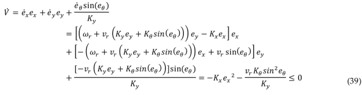
When a scalar function V is proposed as a Lyapunov function candidate for the system:

Clearly, and , thus the Equation (38) above is a positive definite function. By Lemma 2:

̇ ̇ ̇ ̇ ( )

*( ( ( ))) + * ( ( ( ))) ( )+

[ ( ( ))] ( )

₍₃₉₎

Consequently the Lyapunov function V’s derivative is a negative definite function. That means uniformly asymptotically stability around under the conditions that are are bounded and , are continuous. The above Lyapunov stability analysis and controller are used in reference (Kanayama et al., 1990).

SYSTEM SIMULATION

In Figure 3, general description of systems and controllers were shown below :

Figure 3. Control block diagram

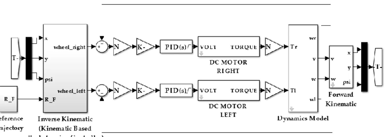
The PID controller that is shown in the Figure 4 is used to control volt inputs for the DC motors. The simulation block diagram that is based on the general diagram was shown below:

Re ference Traje ctory Kine matic Base d Backste pping Controlle r DC Motor Mobile Robot Forward Kine matics 𝑞 𝑥 𝑦 𝜃 𝑞𝑟 𝑞 𝜔 𝜏 𝑉 𝜔𝑒

Figure 4. Simulation block diagram

Figure 5. KBBC block diagram

Table 1. Parameters For Robot and DC-Motors

Robot DC-Motor

Term Unit Value Term Unit Value

27 ( ) 0.5 ( ) 0.732 0.0025 ⁄ _0.0012 0.05 ⁄ ( ) - ( ) 6640

Numerical values of imposed constraints are;

e e ⁄ e e ⁄

In the following simulations; initial values for linear and angular velocities are selected as 0. The simulation time t = 65 seconds, the angular speed for the trajectory w = 0.1 rad/s, the scale factor k = 1.5 meter. The square trajectory general equation defined as below for (x, y, θ) is (0, 0, 0);

( ( )) ( ) ( ( )) ( ) (40) RESULT AND DISCUSSION

Trajectory following results for without the PID controller and with the PID controller are considered below . The PID controller parameters are tuned as . For graphically presented initial pose [x, y, θ] for the first condition is [0, 0, 0], for the second condition is [0, 0, pi/2], for the third condition is [0, 0, pi/2].

Figure 6. Controllers with starting position [0, 0, 0].

In the Figure 6, the results show that after applying the PID controller to the kinematic based backstepping controller; settling time decrease. Also, decereasing of error were observed at small rate.

Figure 7. Controllers with starting position [0, 0, pi/2].

In the Figure 7, the results show that after applying the PID controller to the kinematic based backstepping controller; the settling time and overshot decrease significantly. Also, decreasing of the error were observed at the small rate.

Figure 8. Controllers with starting position [0, 0, pi].

In the Figure 8, the results show that after applying the PID controller to the kinematic based backstepping controller; the settling time and overshot decrease significantly. Also, decreasing of the error were observed at the small rate.

For detailed examination, the KBBC Controller’s chosen parameters are without the PID controller and with the PID controller. Controller parameters are tuned as

for PID controller. Initial pose is [0, 1.5, -pi/4].

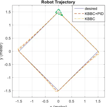
Figure 9. Conrtrollers with starting position [0, 1.5, -pi/4].

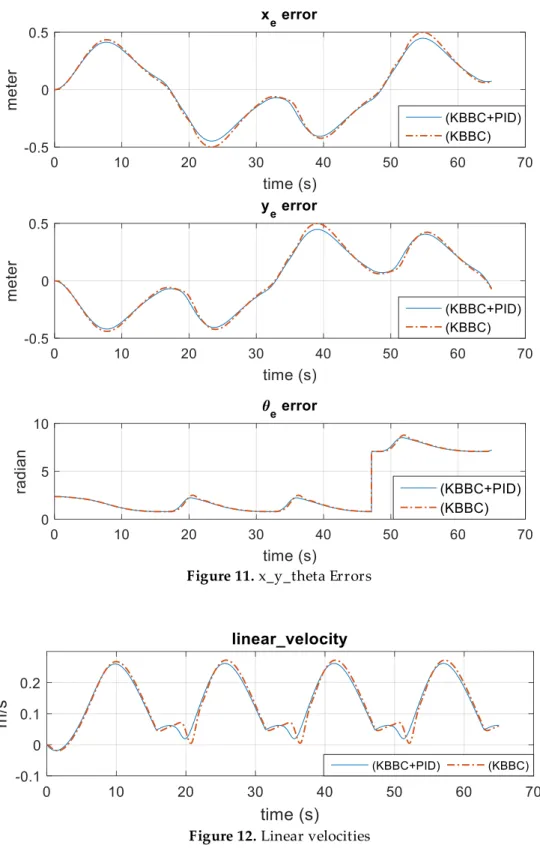
Figure 11. x_y_theta Errors

Figure 12. Linear velocities

In the Figure 9, for the comparison between the KBBC+PID and KBBC minimum errors were chosen. In the Figure 11, differences between controllers’ errors were at the small rate. In the Figure 10, for the KBBC, it can be said that it needs more torque than the KBBC+PID. At the 15.71, 31.42 , 47.13, 62.84 seconds for both DC motors instantaneous change at the torque rate for the KBBC+PID. As estimated, in the Figure 12, a sudden change in the linear velocity can be seen at the same times for the KBBC+PID.

CONCLUSION

In this present study, a differential drive mobile robot dynamic equations were derived by Lagrange method. The stable control method, capable of dealing with the tracking square trajectory of the differential drive mobile robot, had been derived using the kinematic based backstepping controller and had been combined with the PID controller for the DC motors. The square shaped trajectory was selected. Simulations were performed by with the proposed control law using Matlab/Simulink. The validity of the proposed controller was proved by Lyapunon function. The proposed controller (KBBC+PID) showed a good tracking performance and stability for the different initial positon. Obtained results showed that the proposed controller can be developed effectively by the tuning parameters. ACKNOWLEDGE

This article was derived and supported from Faik DEMİRBAŞ’s master thesis ’’Trajectory Tracking Control of an Obstacle Avoiding Mobile Robot’’.

REFERENCES

Ali, R. S., Aldair, A. A., Almousawi, A. K., 2014, ‘’Design an Optimal PID Controller using Artificial Bee Colony and Genetic Algorithm for Autonomous Mobile Robot’’, International Journal of Computer Applications (0975 – 8887), Vol. 100 (1), pp. 8-16.

Dhaouadi, R., Hatab, A. A., 2013, ‚Dynamic Modelling of Differential-Drive Mobile Robots using Lagrange and Newton-Euler Methodologies: A Unified Framework‛, Research Article, Advances in Robotics & AutomationTechnology, Vol. 2 (2), pp. 1-7.

España Cabrera, A., 2014, Rapid Prototyping of Mobile Robot Control Algorithms, Degree of Master of Science in Faculty of Electrical Engineering, Department of Control Engineering, Czech Technical University In Prague.

Fierro, R., Lewis, F. L., ‚Control of A Nonholonomic Mobile Robot: Backstepping Kinematics Into Dynamics,‛ in Proceedings of 34th IEEE Conference on Decision and Control, New Orleans, Louisiana, USA, pp. 3805-3810, 13-15 December 1995.

Hwang, E. J., Kang, H. S., Hyun C. H., Park, M., 2013, ‘’Robust Backstepping Control Based on a Lyapunov Redesign for Skid-Steered Wheeled Mobile Robots’’, International Journal of Advanced Robotic Systems, Vol.10, 26.

Kanayama, Y., Kimura, Y., Miyazaki, F., Noguchi, T., ‚A Stable Tracking Control Method for An Autonomous Mobile Robot,‛ in Proc. IEEE International Conference on Robotics and Automation, Cincinnati, Ohio, pp. 384–389, 13-18 May 1990.

Mac, T. T., Copot, C., De Keyser, R., Tran T. D., Vu, T., 2016, ‘’MIMO Fuzzy Control for Autonomous Mobile Robot’’, Journal of Automation and Control Engineering, Vol. 4 (1), pp. 65-70.

Mohareri, O., 2009, Mobile Robot Trajectory Tracking Using Neural Networks, Degree of Master of Science in Mechatronics Engineering, American University of Sharjah, United Arab Emirates.

Oubbati, M., Schanz, M., Levi, P., ‚Kinematic and Dynamic Ada ptive Control of A Nonholonomic Mobile Robot Using A RNN‛, in Proceedings of IEEE International Symposium on Computational Intelligence in Robotics and Automation (CIRA '05), Espoo, Finland, pp. 27–33, 27-30 Jun 2005. Sidek, S. N., 2008, Dynamic Modeling and Control of Nonholonomic Wheeled Mobile Robot Subjected to Wheel

Slip, Degree of Doctor OF Philosophy in Faculty of the Graduate School, Department of Electrical Engineering, Vanderbilt University.

Solea, R., Filipescu, A., Filipescu Jr., A., Minca, E., Filipescu, S., ‘’Wheelchair Control and Navigation Based on Kinematic Model and Iris Movement Robots’’, 2015 IEEE 7th International Conference on Cybernetics and Intelligent Systems (CIS) and IEEE Conference on Robotics, Automation and Mechatronics (RAM), Angkor Wat, Cambodia, pp. 78-83,15-17 July 2015.

Swadi, S. M., Tawfik, M. A., Abdulwahab E. N., Kadhim , H. A., ‘’Fuzzy-Backstepping Controller Based on Optimization Method for Trajectory Tracking of Wheeled Mobile Robot ’’, 2016 UKSim-AMSS 18th International Conference on Computer Modelling and Simulation, Cambridge, United Kingdom, pp. 147-152, 6-8 April 2016.

Tawfik, M. A., Abdulwahb E. N., Swadi, S. M., 2014, ‘‘Trajectory Tracking Control for a Wheeled Mobile Robot Using Fractional Order PID Controller’’, Al-Khwarizmi Engineering Journal, Vol. 10 (3), pp. 39- 52.

Yuan, G., 2001, Tracking Control of A Mobile Robot Using Neural Dynamics Based Approaches, Degree of Master of Science in School of Engineering, University of Guelph, Canada.