Results in Physics 19 (2020) 103409
Available online 1 October 2020
2211-3797/© 2020 The Authors. Published by Elsevier B.V. This is an open access article under the CC BY-NC-ND license (http://creativecommons.org/licenses/by-nc-nd/4.0/).
Construction of exact traveling wave solutions of the Bogoyavlenskii
equation by (G
′/
G, 1/G)-expansion and (1/G
′)
-expansion techniques
Asíf Yokus
a, Hülya Durur
b, Hijaz Ahmad
c, Phatiphat Thounthong
d, Ying-Fang Zhang
e,* aDepartment of Actuary, Faculty of Science, Firat University, Elazig 23200, TurkeybDepartment of Computer Engineering, Faculty of Engineering, Ardahan University, Ardahan 75000, Turkey cDepartment of Basic Sciences, University of Engineering and Technology, Peshawar 25000, Pakistan
dRenewable Energy Research Centre, Department of Teacher Training in Electrical Engineering, Faculty of Technical Education, King Mongkut’s University of Technology
North Bangkok, 1518 Pracharat 1 Road, Bangsue, Bangkok 10800, Thailand
eSchool of Mathematics and Information Science, Henan Polytechnic University, Jiaozuo 454000, China
A R T I C L E I N F O Keywords:
(1/G′
)-expansion technique Traveling wave solutions The Bogoyavlenskii equation Expansion method Exact solution
A B S T R A C T
In this article, we construct exact solutions of the Bogoyavlenskii equation using (1/G′
)-expansion and (G′/G, 1/G)-expansion techniques. Both techniques have been successfully implemented to obtain exact solutions including hyperbolic, complex trigonometric, trigonometric and rational solutions of the Bogoyavlenskii equa-tion. 3D, contour and 2D graphics are presented of the solutions obtained for different special values. Further, the advantages and disadvantages of both the techniques have been discussed in this study. The proposed techniques are reliable and applicable for attaining wave solutions of nonlinear differential equations. Also, these techniques can greatly minimize the size of computing work compared to other available techniques.
1. Introduction
Nonlinear partial differential equations (nPDEs) are absolutely essential to progress in the study of all scientific & engineering disci-plines, including physics, engineering & chemistry. nPDEs are formu-lated from first principles to accurately describe key underlying features of what is being studied, whether it be fluid-, orbital-, structural-, aero-, or other mechanics or mechanisms. The solution to such nPDEs, either in closed form (if possible), or by brute force (if necessary, using com-puters), provide the answers to important scientific questions that enable progress in confidently understanding the complex phenomena being studied. Analytical solutions of these equations are of great importance in many physical phenomena, such as applied mechanics, fluid dynamics, finance, solid state physics, astronomy, plasma physics, computational mechanics and hydrodynamics. In the last few decades, many new techniques have been applied for finding these solutions, e.g.,
modified exp( − Ω(ζ))-expansion function technique [1,2], parameter
expansion technique [3], (1/G′
)-expansion technique [4,5], auxiliary
equation method [6,7], Homotophy analysis technique [8],
Sine–Gordon expansion technique [9], trigonometric function series
method [10,11], modified mapping method [12], modified
trigono-metric function series method [13], bifurcation method [14], modified
(G′/G)-expansion technique [16,15], meshfree techniques [17–19],
multiple scales Homotopy perturbation technique [20], local meshless
method [21,22], sub equation technique [23], Adomian’s
decomposi-tion technique [24], new sub equation technique [25], variational
iteration algorithm-I [26–29], variational principle [30–32], Laplace
transform technique [33,34], ricatti transformation method [35]
vari-ational iteration technique [36–38], variational iteration algorithm-II
[39–43], Hamiltonian approach [44,45], homotopy perturbation
tech-nique [46–48] and other procedures [49–58].
The main aim of the current paper is to construct the exact solutions of the Bogoyavlenskii equation by using these two different expansion
techniques. Consider the Bogoyavlenskii equation [59]:
4ut+uxxy − 4u2uy− 4uxv = 0,
uuy=vx. (1)
There are a variety studies related to the Bogoyavlenskii equation. For example; Malik et al. investigated the Bogoyavlenskii equation by
applying (G′
/G)-expansion technique [59], analytical solutions of the
Bogoyavlenskii equation are obtained by applying the singular manifold
technique and the traveling wave technique by Peng and Shen [60].
Modified extended tanh-function technique utilized by Zahran et al.
[61] to obtained analytical solution of the Bogoyavlenskii equation. Yu * Corresponding author.
E-mail address: [email protected] (Y.-F. Zhang).
Contents lists available at ScienceDirect
Results in Physics
journal homepage: www.elsevier.com/locate/rinp
https://doi.org/10.1016/j.rinp.2020.103409
and Sun [62] applied modified technique of simplest equation for the analytical treatment of the Bogoyavlenskii equation.
The remaining portion of this paper is as: In Section 2,
(1/G′)-expansion technique is elaborated, in Section 3, (G′/G,
1/G)-expansion technique is discussed and illustrated. In Section 4,
(1/G′)-expansion technique is used to obtained traveling wave solutions
of the Bogoyavlenskii equation. In Section 5, applications of (G′
/G,
1/G)-expansion technique are discussed and utilized to solve the Bogoyavlenskii equation, applicability and reliability of the proposed techniques are shown through 3D, contour and 2D graphics. Conclusion is discussed in the last section.
2. (1/G′
)-expansion technique
Consider a general form of the following nonlinear PDE,
σ ( u,∂u ∂t, ∂u ∂x, ∂u ∂y, ∂2 u ∂x2,… ) =0. (2)
Here, let u = U(ζ) = u(x, y, t),v = V(ζ) = v(x, y, t), ζ = x + y − ct,
c ∕= 0, where c is a constant and the speed of the wave. We can convert it into the following nODE for U(ζ)
τ(U, U′,U′′,
…) = 0, (3)
where prime refers to derivatives related to ζ. The solution of Eq. (4) is
assumed to have the form
u(ζ) = a0+ ∑n i=1 ai ( 1 G′ (ζ) )i , (4)
whereas ai, (i = 0, 1, …, n) are constants, n is the balancing term and is
an integer, G = G(ζ) provides the following second order IODE
G′′+κG′
+μ=0, (5)
where μand κare constants to be determined after,
1
G′ (ζ)=
1
− μκ+Acosh(ζκ) − Asinh(ζκ), (6)
where A is integral constant. If the desired derivatives of the Eq. (4) are
calculated and substituting in the Eq. (3), a polynomial with the
argu-ment (1/G′
)is attained. An algebraic equation system is created by
equalizing the coefficients of this polynomial to zero. The equation are
solved using package program and put into place in the default Eq. (3)
solution function. Lastly, the solutions of Eq. (1) are found.
3. (G′
/G, 1/G)-expansion technique
Consider a general form of NLEEs containing two or more arguments to be analyzed is written as follows:
Z(u, ut,ux,uy,utt,uxx,… )
=0. (7)
If u = U(ζ) = u(x, y, t), v = V(ζ) = v(x, y, t), ζ = x +y − ct
trans-mutation is applied in Eq. (7), Eq. (7) is converted into a NLODE and this
equation may usually be written as:
z(U′,U′′,
U′′′,…) = 0. (8)
where prime refers to derivatives related to ζ. Complexity can be
reduced by integrating Eq. (8). By the nature of this technique, G = G(ζ)
provides the following second order IODE
G′′(ζ) + κG(ζ) =μ. (9)
Furthermore, to provide operational aesthetics as ϕ = ϕ(ζ) = G′
(ζ)/ G′
(ζ)GG(ζ) and ψ=ψ(ζ) =1/1G(ζ)G(ζ) We may write derivatives of
functions defined here;
ϕ′= − ϕ2+μψ− κ,ψ′
= − ϕψ. (10)
We can offer the behavior of solution function Eq. (9) according to
the state of κ, taking into account the equations given by the Eq. (10).
i: If κ < 0 G(ζ) = c1sinh( ̅̅̅̅̅̅ − κ √ ζ) + c2cosh( ̅̅̅̅̅̅ − κ √ ζ) +μ κ, (11)
whereas c1 and c2 are reel numbers. Considering Eq. (11),
ψ2= − κ κ2σ+μ2 ( ϕ2− 2μψ+κ),σ=c2 1− c22, (12) Eq. (12) is written. ii: If κ > 0 G(ζ) = c1sin ( ̅̅̅ κ √ ζ ) +c2cos ( ̅̅̅ κ √ ζ ) +μ κ, (13)
here c1 and c2 are reel numbers. Considering Eq. (13),
ψ2= κ κ2σ− μ2 ( ϕ2− 2μψ+κ),σ=c2 1+c22, (14) is written. iii: If κ = 0 G(ζ) =μ 2ζ 2+c 1ζ + c2, (15)
here c1 and c2 are reel numbers. Considering Eq. (15),
ψ2= 1
c2 1− 2μc2
(
ϕ2− 2μψ), (16)
is written. In terms of ϕ and ψ polynomials, solution of Eq. (8) is
u(ζ) =∑ n i=0 aiϕi+ ∑n i=1 biϕi− 1ψ. (17)
Wherein, ai(i = 0, 1, …, n) and bi(i = 1, …, n) counts then are
con-stants to be find out. n is a positive equilibrium term that may be ob-tained by comparing the maximum order derivative and the maximum order nonlinear term in Eq. (13). If Eq. (17) is written in Eq. (8) with Eqs.
(10), (12), (14) or (16), a polynomial function associated with ϕ and ψ is
written. Each term coefficient of ϕiψj(i = 0, 1, …, n) (j = 1, …, n) of the
attained polynomial functions are equated to zero and a system alge-braic equations is obtained for ai,bi,c,μ,c1,c2 and κ (i = 0, 1, …, n). The
necessary coefficients are attained by solution of the algebraic equation with help of built in computer-package programs. Obtained coefficients
are written in Eq. (17) and U(ζ) solution function of Eq. (8) is obtained
and if ζ = x +y − ct transmutation is implemented in the reverse order, we will attain analytic solution u(x, y, t) of Eq. (7).
4. Application of (1/G′
)-expansion technique
We take Eq. (1) and using transformation
u = U(ζ) = u(x, y, t), v = V(ζ) = v(x, y, t), ζ = x +y − ct, c represents
the velocity of the traveling wave, we obtain − 4cU′+U′′′− 4U2U′
− 4U′V = 0,
V = U2/U22 , (18)
in Eq. (18), the second equation is written in the first equation and once
integral is taken
U′′− 2U3− 4cU = 0. (19)
In Eq. (19), we get term n = 1 from the definition of balancing term
and the following situation is obtained in Eq. (4),
U(ζ) = a0+a1 ( 1 G′ (ζ) ) , a1 ∕= 0, (20)
where a0,a1 unknown constants to be find out later. Eq. (20) into Eq.
(19) and coefficients are equal to zero, we may establish the following algebraic equation systems
Const : − 4ca0− 2a30=0, ( 1 G′ [ζ] )1 : − 4ca1+κ2a1− 6a20a1=0, ( 1 G′ [ζ] )2 : 3κμa1− 6a0a21=0, ( 1 G′ [ζ] )3 :2μ2a 1− 2a31=0. (21) Case I. a0= − κ 2, c = − κ2 8, μ= − a1, (22)
replacing values Eq. (22) into Eq. (20) and attain the following
hyper-bolic exact solutions for Eq. (1):
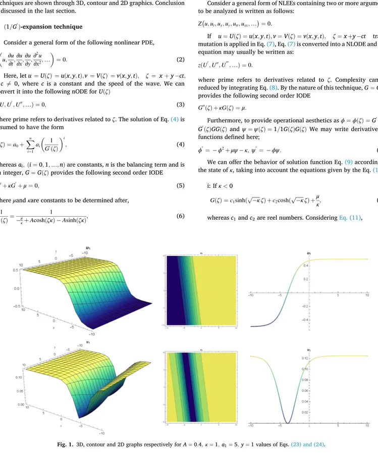
u1(x, y, t) = − κ 2+ a1 Acosh [ κ ( x + y +tκ2 8 ) ] − Asinh [ κ ( x + y +tκ2 8 ) ] +a1 κ , (23) v1(x, y,t) = 1 2 ⎛ ⎜ ⎜ ⎝ − κ 2+ a1 Acosh [ κ ( x + y +tκ2 8 ) ] − Asinh [ κ ( x + y +tκ2 8 ) ] +a1 κ ⎞ ⎟ ⎟ ⎠ 2 . (24)
The hyperbolic exact solutions of Eqs. (23) and (24) produced from
the (1/G′
)-expansion technique is as in Fig. 1.
Case II. a0= − i ̅̅̅ 2 √ ̅̅̅ c √ , a1= − μ, κ = 2i ̅̅̅ 2 √ ̅̅̅ c √ , (25)
replacing values Eq. (25) into Eq. (20) and get the following complex
trigonometric wave solution for Eq. (1):
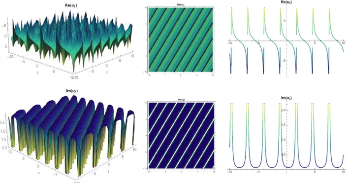
u2(x, y, t) = − i ̅̅̅ 2 √ ̅̅̅ c √ − iμ μ 2√̅̅2√̅̅c+Acos [ 2√̅̅̅2√̅̅̅c( − ct + x + y)]− iAsin[2√̅̅̅2√̅̅̅c( − ct + x + y)], (26) v2(x, y, t) = 1 2 ⎛ ⎜ ⎜ ⎝ − i ̅̅̅ 2 √ ̅̅̅ c √ − iμ μ 2√̅̅2√̅̅c+Acos [ 2√̅̅̅2√̅̅̅c( − ct + x + y)]− iAsin[2√̅̅̅2√̅̅̅c( − ct + x + y)] ⎞ ⎟ ⎟ ⎠ 2 . (27)
The complex trigonometric wave solution of Eqs. (26) and (27)
produced from the (1/G′
)-expansion technique is as in Figs. 2 and 3.
Fig. 2. 3D, contour and 2D graphs respectively for A = 0.4,μ= −1, c = 0.6, y = 1 values of Eq. (26).
5. Applications (G′
/G, 1/G)-expansion technique
In Eq. (19), we get n = 1 from the definition of balancing term and
the following situation is obtained in Eq. (17),
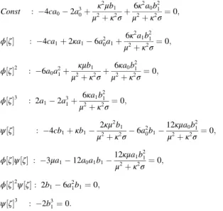
u(ζ) = a0+a1ϕ[ζ] + b1ψ[ζ], (28)
replacing Eq. (28) into Eq. (19) and the coefficients are equal to zero, we
may establish the following algebraic equation systems
Const : − 4ca0− 2a30+ κ2μb 1 μ2+κ2σ+ 6κ2a 0b21 μ2+κ2σ=0, ϕ[ζ] : − 4ca1+2κa1− 6a20a1+ 6κ2a 1b21 μ2+κ2σ=0, ϕ[ζ]2 : − 6a 0a21+ κμb1 μ2+κ2σ+ 6κa0b21 μ2+κ2σ=0, ϕ[ζ]3 : 2a 1− 2a31+ 6κa1b21 μ2+κ2σ=0, ψ[ζ] : −4cb1+κb1− 2κμ2b 1 μ2+κ2σ− 6a20b1− 12κμa0b21 μ2+κ2σ=0, ϕ[ζ]ψ[ζ] : − 3μa1− 12a0a1b1− 12κμa1b21 μ2+κ2σ=0, ϕ[ζ]2ψ[ζ] : 2b1− 6a21b1=0, ψ[ζ]3 : − 2b3 1=0. (29)
The aim with ready computer package program has been achieved and we conclude with the following remarks:
If κ < 0, Case I:
a0=0, a1= − 1, b1=0, c =
κ
2, μ=0, (30)
replacing values Eq. (30) into Eq. (28) and attain the following
hyper-bolic exact solutions for Eq. (1):
u3(x,y,t) = − c2 ̅̅̅̅̅̅ − κ √ cosh[ ̅̅̅̅̅̅√− κ ( x + y − tκ 2 )] +c1 ̅̅̅̅̅̅ − κ √ sinh[ ̅̅̅̅̅̅√− κ ( x + y − tκ 2 )] c1cosh [ ̅̅̅̅̅̅ − κ √ ( x + y − tκ 2 )] +c2sinh [ ̅̅̅̅̅̅ − κ √ ( x + y − tκ 2 )] , (31) v3(x,y,t)= ( c2 ̅̅̅̅̅̅ − κ √ cosh[ ̅̅̅̅̅̅√− κ ( x+y− tκ 2 )] +c1 ̅̅̅̅̅̅ − κ √ sinh[ ̅̅̅̅̅̅√− κ ( x+y− tκ 2 )])2 2 ( c2cosh [ ̅̅̅̅̅̅ − κ √ ( x+y− tκ 2 )] +c2sinh [ ̅̅̅̅̅̅ − κ √ ( x+y− tκ 2 )])2 . (32)
The hyperbolic exact solutions of Eqs. (31) and (32) produced from
the (G′
/G, 1/G)-expansion technique is as in Fig. 4.
If κ > 0, Case II:
a0=0, a1= − 1, b1=0, μ=0, c =
κ
2, (33)
replacing values Eq. (33) into Eq. (28) and attain the following
trigo-nometric exact solutions for Eq. (1):
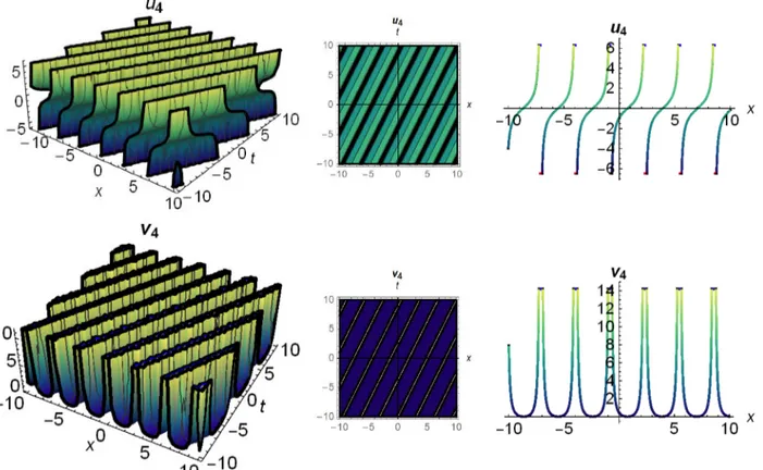
u4(x, y, t) = − c2 ̅̅̅ κ √ cos[ ̅̅̅√ (κ x + y − tκ 2 ) ] − c1 ̅̅̅ κ √ sin[ ̅̅̅√ (κ x + y − tκ 2 ) ] c1cos [ ̅̅̅ κ √ ( x + y − tκ 2 ) ] +c2sin [ ̅̅̅ κ √ ( x + y − tκ 2 ) ] , (34) v4(x, y, t) = ( c2 ̅̅̅ κ √ cos[ ̅̅̅√ (κ x + y − tκ 2 ) ] − c1 ̅̅̅ κ √ sin[ ̅̅̅√ (κ x + y − tκ 2 ) ] )2 2 ( c1cos [ ̅̅̅ κ √ ( x + y − tκ 2 ) ] +c2sin [ ̅̅̅ κ √ ( x + y − tκ 2 ) ] )2 . (35)
The trigonometric exact solutions of Eqs. (34) and (35) produced from the (G′
/G,1/G)-expansion technique is as in Fig. 5.
Fig. 5. 3D, contour and 2D graphs respectively for κ = 1, y = 1, c1=1, c2=3 values of Eqs. (34) and (35).
If κ = 0, Case III:
a0=0, a1=1, b1=0, c = 0, μ=0, (36)
replacing values Eq. (36) into Eq. (28) and attain the following rational
exact solutions for Eq. (1):
u5(x, y, t) = c2 c1+c2(x + y) , (37) v5(x, y, t) = c22 2(c1+c2(x + y) )2 . (38)
The rational exact solutions of Eqs. (37) and (38) produced from the
(G′/G,1/G)-expansion technique is as in Fig. 6.
6. Results and discussion
Both techniques are effective and powerful techniques for solving
partial differential equations. In terms of the solutions it produces, (G′
/G,
1/G)-expansion technique offers more solutions. These solutions vary depending on the condition of the κ. In terms of transaction density, we can say that (1/G′
)-expansion technique is more advantageous. This
situation can be seen in the systems of Eqs. (21) and (29) obtained in the
application of the techniques, which Eq. (21) is simpler than the Eq.
(29). What is scientifically beautiful is that both techniques offer
different types of solutions. If we examine both techniques in terms of the balancing term, we can conclude that as the balancing term grows,
the transaction complexity in the (G′
/G,1/G)- expansion technique will
become even more intense. When the constants in the solutions obtained in this study gain physical meaning, it will be much more valuable. This may be important to the solutions produced for us scientists working in physical practice. Consequently, both techniques can be recommended to get solutions of nonlinear partial differential equations.
7. Conclusions
In this letter, (G′
/G,1/G)-expansion and (1/G′)-expansion techniques were used for obtaining different type traveling wave solutions of the Bogoyavlenskii equation. Both techniques are effective and powerful in obtaining solutions of (nPDEs). Both techniques were applied success-fully and the data obtained were presented, the ready computer package program is utilized for graphics and computations. By applying these techniques to the Bogoyavlenskii equation, different type traveling wave solutions hyperbolic, complex trigonometric, trigonometric and rational solutions are obtained. For the solutions found 3D, contour and 2D graphics are presented for different values given to the constants. Furthermore, the applied techniques are effective, powerful and can be used in future works to establish new exact solutions of many other nonlinear differential equations.
Funding
The research was supported by the National Natural Science Foun-dation of China (Grant No. 11501170).
Declaration of Competing Interest
The authors declare that they have no known competing financial interests or personal relationships that could have appeared to influence the work reported in this paper.
References
[1] Sulaiman TA, Bulut H, Yokus A, Baskonus HM. On the exact and numerical solutions to the coupled Boussinesq equation arising in ocean engineering. Indian J Phys 2019;93(5):647–56.
[2] Yokus A, Baskonus HM, Sulaiman TA, Bulut H. Numerical simulation and solutions of the two-component second order KdV evolutionarysystem. Numer Methods Partial Differ Equ 2018;34(1):211–27.
[3] Sedighi HM, Shirazi KH. Vibrations of micro-beams actuated by an electric field via parameter expansion method. Acta Astronaut 2013;85:19–24.
[4] Yokus¸ A, Durur H. Complex hyperbolic traveling wave solutions of Kuramoto- Sivashinsky equation using (1/G′
)expansion method for nonlinear dynamic theory. Balíkesir Üniversitesi Fen Bilimleri Enstitüsü Dergisi 2019;21(2):590–9. [5] Durur H, Yokus A. (1/G′
)-Açílím Metodunu Kullanarak Sawada-Kotera Denkleminin Hiperbolik Yürüyen Dalga Ǩozümleri. Afyon Kocatepe Üniversitesi Fen Ve Mühendislik Bilimleri Dergisi 2019;19(3):615–9.
[6] Zayed EM, Al-Nowehy AG. New extended auxiliary equation method for finding many new Jacobi elliptic function solutions of three nonlinear Schr¨odinger equations. Waves in Random and Complex Media 2017;27(3):420–39. [7] Jiong S. Auxiliary equation method for solving nonlinear partial differential
equations. Phys Lett A 2003;309(5–6):387–96.
[8] Abbasbandy S, Zakaria FS. Soliton solutions for the fifth-order KdV equation with the homotopy analysis method. Nonlinear Dyn 2008;51(1–2):83–7.
[9] Korkmaz A, Hepson OE, Hosseini K, Rezazadeh H, Eslami M. Sine-Gordon expansion method for exact solutions to conformable time fractional equations in RLW-class. J King Saud Univ – Sci 2018.
[10] Zhang Z-Y. New exact traveling wave solutions for the nonlinear Klein-Gordon equation. Turkish J Phys 2008;32(5):235–40.
[11] Zhang Z-Y. Exact traveling wave solutions of the perturbed Klein-Gordon equation with quadratic nonlinearity in (1+1)-dimension, Part I: Without local inductance and dissipation effect. Turkish J Phys 2013;37(2):259–67.
[12] Zhang Z-Y, Liu Z-H, Miao X-J, Chen Y-Z. New exact solutions to the perturbed nonlinear Schr¨odinger’s equation with Kerr law nonlinearity. Appl Math Comput 2010;216(10):3064–72.
[13] Zhang Z-Y, Li X-X, Liu Z-H, Miao X-J. New exact solutions to the perturbed nonlinear Schrodingers equation with Kerr law nonlinearity via modified trigonometric function series method. Commun Nonlinear Sci Numer Simul 2011; 16(8):3097–106.
[14] Zhang Z-Y, Liu Miao XJ, Chen YZ. Qualitative analysis and traveling wave solutions for the perturbed nonlinear Schr¨odinger’s equation with Kerr law nonlinearity. Phys Lett A 2011;375(10):1275–80.
[15] Yokus A, Durur H, Ahmad H, Yao S-W. Construction of different types analytic solutions for the Zhiber-Shabat equation. Mathematics 2020;8(6):908. [16] Miao X-J, Zhang Z-Y. The modified (G′
/G)-expansion method and traveling wave
solutions of nonlinear the perturbed nonlinear Schr¨odinger’s equation with Kerr law nonlinearity. Commun Nonlinear Sci Numer Simul 2011;16(11):4259–67. [17] Khan MN, Siraj-ul-Islam I, Hussain I, Ahmad H Ahmad. A local meshless method
for the numerical solution of space-dependent inverse heat problems. Math Meth Appl Sci 2020. https://doi.org/10.1002/mma.6439.
[18] Khan MN, Ahmad I, Ahmad H. A radial basis function collocation method for space-dependent inverse heat problems. J Appl Comput Mech 2020. https://doi. org/10.22055/jacm.2020.32999.2123.
[19] Srivastava HM, Ahmad H, Ahmad I, Thounthong P, Khan MN. Numerical simulation of three-dimensional fractional-order convection-diffusion PDEs by a local meshless method. Thermal Sci 2020.
[20] El-Dib Y. Stability analysis of a strongly displacement time-delayed duffing oscillator using multiple scales Homotopy perturbation method. J Appl Comput Mech 2018;4(4):260–74.
[21] Ahmad I, Khan MN, Inc M, Ahmad H, Nisar KS. Numerical simulation of simulate an anomalous solute transport model via local meshless method. Alexandria Eng J 2020.
[22] Ahmad I, Ahmad H, Thounthong P, Chu Y-M, Cesarano C. Solution of multi-term time-fractional PDE models arising in mathematical biology and physics by local meshless method. Symmetry 2020;12(7):1195.
[23] Durur H, Tasbozan O, Kurt A, S¸enol M. New wave solutions of time fractional Kadomtsev-Petviashvili equation arising in the evolution of nonlinear long waves of small amplitude. Erzincan Üniversitesi Fen Bilimleri Enstitüsü Dergisi 2019;12 (2):807–15.
[24] Kaya D, Yokus A. A numerical comparison of partial solutions in the decomposition method for linear and nonlinear partial differential equations. Math Comput Simul 2002;60(6):507–12.
[25] Kurt A, Tasbozan O, Durur H. The exact solutions of conformable fractional partial differential equations using new sub equation method. Fundam J Math Appl 2019; 2(2):173–9.
[26] Ahmad H, Rafiq M, Cesarano C, Durur H. Variational iteration algorithm-I with an auxiliary parameter for solving boundary value problems. Earthline J Math Sci 2020;3(2):229–47.
[27] Ahmad H, Khan TA, Cesarano C. Numerical solutions of coupled burgers equations. Axioms 2019;8(4):119.
[28] He J-H. A short review on analytical methods for a fully fourth-order nonlinear integral boundary value problem with fractal derivatives. Int J Numer Methods Heat Fluid Flow 2020. ahead-of-print.
[29] Ahmad H, Khan TA, Stanimirovic P, Ahmad I. Modified variational iteration technique for the numerical solution of fifth order KdV type equations. J Appl Comput Mech 2020. https://doi.org/10.22055/jacm.2020.33305.2197. [30] He J-H. Variational principle for the generalized KdV-burgers equation with fractal
derivatives for shallow water waves. J Appl Comput Mech 2020;6(4). [31] He JH. Generalized variational principles for buckling analysis of circular
cylinders. Acta Mech 2019;231(3):899–906.
[32] He J-H, Sun C. A variational principle for a thin film equation. J Math Chem 2019; 57(9):2075–81.
[33]Abouelregal AE, Ahmad H. A modified thermoelastic fractional heat conduction model with a single-lag and two different fractional-orders. J Appl Computat Mech 2020.
[34]Abo-Dahab SM, Abouelregal AE, Ahmad H. Fractional heat conduction model with phase lags for a half-space with thermal conductivity and temperature dependent. Math Methods Appl Sci 2020.
[35]Bazighifan O, Ahmad H, Yao S-W. New oscillation criteria for advanced differential equations of fourth order. Mathematics 2020;8(5):728.
[36]He J-H, Latifizadeh H. A general numerical algorithm for nonlinear differential equations by the variational iteration method. Int J Numer Methods Heat Fluid Flow 2020.
[37]Ahmad H, Khan TA, Yao S-W. An efficient approach for the numerical solution of fifth-order KdV equations. Open Math 2020;18(1):738–48.
[38]Anjum N, He J-H. Laplace transform: making the variational iteration method easier. Appl Math Lett 2019;92:134–8.
[39]Ahmad H, Seadawy AR, Khan TA. Numerical solution of Korteweg-de Vries-Burgers equation by the modified variational Iteration algorithm-II arising in shallow water waves. Phys Scr 2019;95(4).
[40]Ahmad H. Auxiliary parameter in the variational iteration algorithm-II and its optimal determination. Nonlinear Sci Lett A 2018;9(1):62–72.
[41]Ahmad H, Seadawy AR, Khan TA, Thounthong P. Analytic approximate solutions for some nonlinear Parabolic dynamical wave equations. J Taibah Univ Sci 2020; 14(1):346–58.
[42]Ahmad H. Variational iteration algorithm-II with an auxiliary parameter and its optimal determination. Nonlinear Sci Lett A 2018;9(1):62–72.
[43] Ahmad H, Seadawy AR, Khan TA. Study on numerical solution of dispersive water wave phenomena by using a reliable modification of variational iteration algorithm. Math Comp Simulat 2020. https://doi.org/10.1016/j. matcom.2020.04.005.
[44]He J-H. Hamiltonian approach to nonlinear oscillators. Phys Lett Sect A Gen At Solid State Phys 2010;374(23):2312–4.
[45]Xu L, He J-H. Determination of limit cycle by Hamiltonian approach for strongly nonlinear oscillators. Int J Nonlinear Sci Numer Simul 2010;11(12):1097–101. [46]He J-H. Addendum: new interpretation of homotopy perturbation method. Int J
Mod Phys B 2006;20(18):2561–8.
[47]He J-H. Homotopy perturbation method for solving boundary value problems. Phys Lett A 2006;350(1–2):87–8.
[48]He J-H. others, Recent development of the homotopy perturbation method. Topol Methods Nonlinear Anal 2008;31(2):205–9.
[49] Liu J-G, He Y. Abundant lump and lump-kink solutions for the new (3+1)- dimensional generalized Kadomtsev-Petviashvili equation. Nonlinear Dyn 2018; 92:1103–8.
[50] Yin Y-H, Ma W-X, Liu J-G, Lü X. Diversity of exact solutions to a (3+ 1)-dimen-sional nonlinear evolution equation and its reduction. Comput Math Appl 2018;76 (6):1275–83.
[51] Sedighi HM, Shirazi KH, Zare J. An analytic solution of transversal oscillation of quintic non-linear beam with homotopy analysis method. Int J Non Linear Mech 2012;47(7):777–84.
[52] Liu J-G, Zhu W-H, He Y, Wu Y-K. Interaction phenomena between lump and solitary wave of a generalized (3+ 1)-dimensional variable-coefficient nonlinear- wave equation in liquid with gas bubbles. Commun Theor Phys 2020;72(8): 085002.
[53] Ahmad H. Variational iteration method with an auxiliary parameter for solving telegraph equations. J Nonlinear Anal Appl 2018;2018(2):223–32.
[54] Ahmad H, Khan TA, Cesarano C. Numerical solutions of coupled Burgers’ equations. Axioms 2019;8(4):119.
[55] Ahmad H, Khan TA, Yao S. Numerical solution of second order Painlev´e differential equation. J Math Comput SCI-JM 2020;21(2):150–7.
[56] Sulaiman TA, Yavuz M, Bulut H, Baskonus HM. Investigation of the fractional coupled viscous Burgers’ equation involving Mittag-Leffler kernel. Physica A Stat Mech Appl 2019;527:121126 .
[57] Ahmad H, Khan TA. Variational iteration algorithm I with an auxiliary parameter for the solution of differential equations of motion for simple and damped mass- spring systems. Noise Vibr Worldwide 2020;51(1–2):12–20.
[58] Ahmad H, Khan TA, Durur H, Ismail GM, Yokus A. Analytic approximate solutions of diffusion equations arising in oil pollution. J Ocean Eng Sci 2020.
[59] Malik A, Chand F, Kumar H, Mishra SC. Exact solutions of the Bogoyavlenskii equation using the multiple (G′
/G)-expansion method. Comput Math Appl 2012;64 (9):2850–9.
[60] Peng YZ, Shen M. On exact solutions of the Bogoyavlenskii equation. Pramana – J Phys 2006;67(3):449–56.
[61] Zahran EHM, Khater MMA. Modified extended tanh-function method and its applications to the Bogoyavlenskii equation. Appl Math Model 2016;40(3): 1769–75.
[62] Yu J, Sun Y. Modified method of simplest equation and its applications to the Bogoyavlenskii equation. Comput Math Appl 2016;72(7):1943–55.