The Time - Varying Natural Rate of Interest and Its
Fundamental Determinants: Time Series Evidence from
Turkey
Ilyas Siklar (Corresponding author) Anadolu University, Eskisehir/Turkey
E-mail: [email protected]
Umit Yildiz
Anadolu University, Eskisehir/Turkey E-mail: [email protected]
Sinan Cakan
Anadolu University, Eskisehir/Turkey E-mail: [email protected]
Received: November 17, 2016 Accepted: December 7, 2016
doi:10.5296/ber.v6i2.10303 URL: http://dx.doi.org/10.5296/ber.v6i2.10303
Abstract
In this study, by estimating the natural rate of interest, its relationship with key macroeconomic variables is analyzed using the time series data obtained from Turkey. As a first step, together with the natural rate of interest, the potential levels of output, prices and foreign exchange rate are estimated by using the Kalman Filter algorithm and then the related gap levels of each variable representing the deviations from their potentials are determined. As a second step of the study, the effects of output, price and exchange rate gaps on the interest rate gap are analyzed by using cointegration and error correction methodologies and the causality relationship among variables are examined. The main conclusion of the current study is that there is significant causality relationship between the interest rate gap, output, price and exchange rate gaps.
1. Introduction
In monetary policy regimes where rate of short-term interest is used as a policy instrument, natural rate of interest plays an important role for identification of the status of monetary policy. As Turkey has been using the short-term interest rate as the fundamental instrument of its monetary policy since 2001, it is a country where monetary policies may be evaluated by estimation of natural rate of interest. When the concept of natural interest is taken as basis, while it is possible to use the gap between the rate of interest used as an instrument by the central bank and the natural rate of interest as a prominent guide for assessment of the current status of the monetary policy, it may also help new monetary policy decisions to be made (Laubach and Williams, 2003).
Although there are several definitions of natural or neutral rates of interest, according to the standard definition that is usually used, it is the short-term rate of interest that allows convergence of production on the potential level without causing instability in the inflation (and by allowing the inflation to be kept at the targeted level) (Bomfim, 1997). Being an unobservable variable is the fundamental problem of the concept of natural interest which, by its definition, offers a very useful and simple use, and bears great importance particularly when central banks use short-term rate of interest as the primary instrument in implementing the monetary policy. Therefore, it is necessary to estimate the natural rate of interest.
The purpose of this study is to forecast the natural rate of interest and the potential levels of macroeconomic variables that possibly affect it. The study also aims to identify the gap level of each variable and to evaluate the relationship among them in the context of Turkey. To this end, the study is made up of 3 parts, in addition to this introduction: literature review; methodology and findings and conclusion. After a brief introduction on the matter in this part of the study, the second part contains a literature review and touches upon prominent studies. A forecast of the natural rate of interest for Turkey will be made and its relation to the variables that affect the rate of interest will be examined in the third part, and fourth part will include a general evaluation of study outcomes.
2. A Short Literature Review
In the literature, a variety of approaches ranging from simple statistical techniques to structural economic models are used to forecast the rates of natural interest. For instance, while Basdenvant et al. (2004) estimates the rate of natural interest for New Zealand using the Hodrick - Prescott multivariable filtering technique, Cuaresma et al. (2003) uses the model of unobservable components in estimating the natural rate of interest for Eurozone. Among the studies that use more complex models such as a dynamic stochastic general equilibrium model include Neiss and Nelson (2001) for the United Kingdom, Giammarioli and Valla (2003) for Eurozone. In the study conducted by Laubach and Williams (2003) for the United States, on the other hand, the trend economic growth rate, natural rate of interest and potential level of production are estimated using semi-structural models through Kalman filter.
the scope of this study.1 In majority of studies in the literature, the natural rate of interest is generally estimated for developed countries and mostly on the basis of a single country. Of these studies, Laubach and Williams (2003) for the United States, Bernhardsen and Gerdrup (2007) for Norway, European Central Bank, ECB, (2004) for Eurozone, Bjorksten and Karagedikli (2003) for New Zealand, Lam and Tkacz (2004) for Canada, Adolfsen et al. (2011) for Sweden stand out. While there is a limited number of studies intended to estimate the natural rate of interest for developing economies, such studies are seen to focus on Latin American countries such as Chile, Colombia and Brazil. The studies that stand out in this respect include Perelli (2012) and Duarte (2010), Portugal and Barcellos (2009), and Minella et al. (2002) for Brazil; Gonzalez et al. (2010; 2012), and Torres (2007) for Colombia; Fuentes and Gredig (2007), and Calderon and Gallego (2002) for Chile; Castillo et al. (2006), Humala and Rodriguez (2009), and Pereda (2010) for Peru. It is fair to say that the study conducted by Öğünç and Batmaz (2012) is one of the few number of studies conducted for Turkey in the literature.
While the natural rate of interest is estimated to be about 2.5% on average for studies conducted for developed economies, it is usually estimated to be about 5% for developing countries, using similar methods. A matter that is emphasized in Laubach and Williams (2003), which is the most cited study among these is that using the natural rate of interest as the key variable in conducting monetary policies is dangerous. In that study, the significant amount of variation observed in the estimated natural rate of interest during the period of study is emphasized, and the following conclusion is reached: "Mismeasurement of the
natural rate of interest by policy decision makers may cause serious deterioration in short run macroeconomic stability."
3. Methodology and Empirical Findings
In this part of the study, by using the time series econometric techniques, natural rate of interest, potential values of each explanatory variable and gap levels (representing the deviations from potential) are estimated. As a last step, the relationship among these gap values are analyzed.
3.1 Dataset
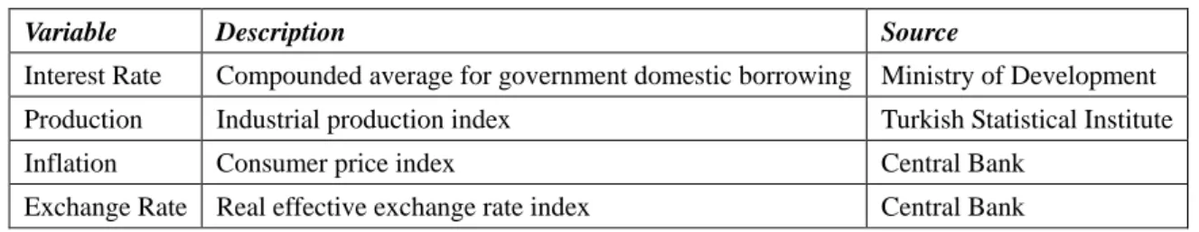
Macroeconomic variables and description of the dataset of each variable are given in Table 1. As can be seen in the Table, the rate of interest is represented by the average rate of compound interest of government’s domestic borrowing and production is represented by industrial production index. On the other hand, consumer price index and real effective exchange rate index are used to indicate the general price level and foreign exchange rate, respectively.
1
Table 1. Macroeconomic Variables
Variable Description Source
Interest Rate Compounded average for government domestic borrowing Ministry of Development Production Industrial production index Turkish Statistical Institute
Inflation Consumer price index Central Bank
Exchange Rate Real effective exchange rate index Central Bank
In determination of potential values of macroeconomic variables, several statistical methods such as linear trend model and Hodrick - Prescott Filter can be used. Kalman Filter which is based on the economic theory and allows time varying values to be found by taking the effect of other economic variables into account, is used in this study to obtain already mentioned potential values.
3.2 Kalman Filter
In statistics and economics, filtering is defined as an algorithm that allows estimation of parameters that cannot be observed and subject to changes in time. The most important property of filtering that distinguishes it from prediction is that while predictions include forecasting for the future, it involves prediction of unobservable variables of the current period (Pasricha, 2010). Kalman Filter was introduced by Rudolf Emil Kalman in his seminal paper titled 'A New Approach to Linear Filtering and Predictions Problems’ in 1960, and it is a linear filtering based on the least squares estimation method (Zarchan et al. 2009:19). At first, this method was used in industrial applications such as video and laser tracking systems, satellite and radar systems, and later in complex simultaneous applications with development of high-speed computers (Chui and Chen, 2009:7). Offering a large area of use in engineering applications, Kalman Filter found itself a place in the studies of statistics and economics intended for identification of optimal levels.
In the literature, Kalman Filter is used for estimation of parameters of equations called as state-space model which is defined as follows (Chui and Chen, 2009:20).
yt = a.xt + εt → measurement equation
xt = xt-1 + ut → transition equation
The model is basically made up of a measurement equation and a transition equation. Here, yt
stands for the equation of observable measurement, and xt the equation of unobservable state.
The transition equation is assumed to be a random walk model formulated according to the AR(1) process. εt and ut represent error terms with zero mean, constant variance and without
serial correlation.
As mentioned earlier, in identifying the potential levels and gap values of macroeconomic variables, Kalman Filter takes into consideration the other explanatory variables based on the economic theory beyond a pure statistical analysis. Therefore, models that include interest rate, production, inflation and foreign exchange rate are needed to determine the potential
levels to be used in this study by this method. To this end, an Aggregate Demand Curve and a Philips Curve model representing the measurement equations of the state-space model is specified. The study of Laubach and Williams’ın (2003) is taken as basis in specifying these models. Therefore, equations resemble to the models used in that study. The Aggregate Demand (IS) and the Philips Curves are stated as follows;
t = ay (l) t-1 + ar (l) ( t-1) + εỹt (1)
t = b (l) t-1 + bỹ (l) t-1 + bx (l) xt-1 + εt (2)
The equation of aggregate demand in equation 1 is formulated with the contribution of lag operator (l). In this equation, represents production gap, in other words, the deviation of the actual production from the potential production. is included in the model as the interest rate gap and shows the difference between the natural rate of interest and monetary interest (average compounded interest rate of government’s domestic borrowing). The natural rate of interest is defined by Wicksell as the nominal rate of interest that ensures stability at the general level of prices and production (Woodford, 2003:25). In equation (1), ay and ar
represent coefficient matrices and εỹt is the error term with the classical properties. As can be
seen in the equation, production gap is a function of its own lagged values and the lagged values of the interest rate gap.
The other equation that we will use in the analysis, namely Philips Curve, is formulated in equation (2) above. In that equation, and x represent inflation and the foreign exchange rate, respectively. b, bỹ and bx indicate coefficient vectors, and εt is the error term with classical
properties. It is assumed in the above specified Philip Curve that inflation is a function of its own lags, lagged values of output gap and the foreign exchange rate.
In this part of the study our main purpose is to determine the deviations of macroeconomic variables in the model from their potential levels and to construct the gap series for each variable to analyze the relationship among them. Therefore, first it will be necessary to determine the potential levels of these macroeconomic variables. In determination of potential values, the Kalman Filter will be implemented to the state-space model as mentioned earlier. Equations (1) and (2) show the measurement equations of the state-space model to which the Kalman Filter is to be applied.
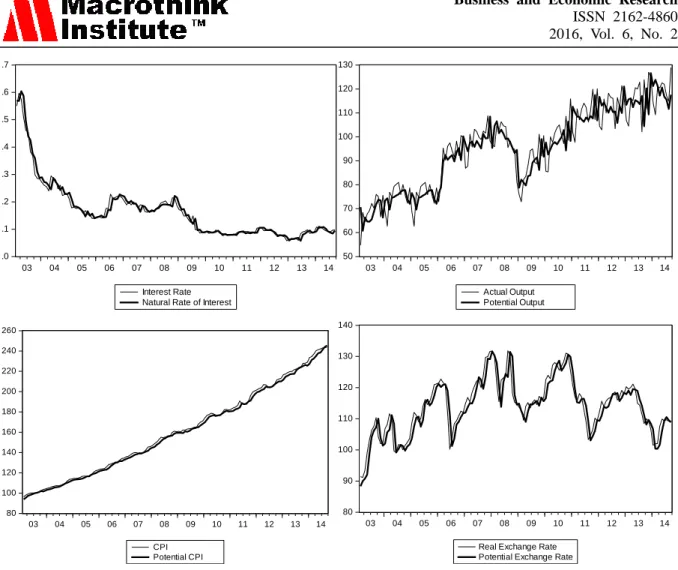
Figure 1 shows the results of macroeconomic variables to which Kalman Filter is applied. The Figure includes the potential levels and actual levels of the rate of interest, production level, consumer price index and real foreign exchange rate. Potential level of the interest rate is also defined as the natural rate of interest.
.0 .1 .2 .3 .4 .5 .6 .7 03 04 05 06 07 08 09 10 11 12 13 14 Interest Rate Natural Rate of Interest
50 60 70 80 90 100 110 120 130 03 04 05 06 07 08 09 10 11 12 13 14 Actual Output Potential Output 80 100 120 140 160 180 200 220 240 260 03 04 05 06 07 08 09 10 11 12 13 14 CPI Potential CPI 80 90 100 110 120 130 140 03 04 05 06 07 08 09 10 11 12 13 14
Real Exchange Rate Potential Exchange Rate
Figure 1. Actual and Potential Levels
The difference between actual and potential levels in the Figure shows how far each variable is from its potential level, in other words, the gap levels of variables.
3.3 Cointegration Analysis
In the econometrics literature, there are many methods for testing the cointegration. Among these methods, implementation of stationary tests to error terms obtained from the cointegration function is a relatively simple method and known as Engel - Granger (EG) or Generalized Engel - Granger Test in the literature (Gujarati and Porter, 2009). In this study, this method is used to test the cointegration relationship among variables. For this purpose, variables are put to an analysis that is basically made up of three steps in order to determine this relationship among variables before estimating the error correction model. These steps are estimation by least squares method of classical regression model that shows the long-term equilibrium relationship among variables; creation of error terms that show deviation from the equilibrium in the estimated long-run model, and testing the unit root for the obtained error terms. In this sense, the regression equation below is estimated with OLS:
In the second step, error terms are obtained by the following equation.
εt = rgt - β0 - β1(ygt) - β2(pgt) - β3(xgt)
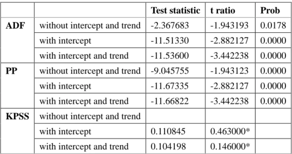
The error terms that are created should not theoretically include unit root, in other words, they should be stationary in order to be used in the error correction model. In order to reach the appropriate result, firstly various unit root tests are conducted for the error terms. For this reason, Augmented Dickey-Fuller (ADF) Unit Root Test, as well as the unit root test of Philips Perron (PP) and Kwiatkowski-Phillips-Schmidt-Shin (KPSS), which are widely used in the literature, are implemented to the residuals.
Table 2. Unit Root Tests Conducted for the Error Term
Test statistic t ratio Prob ADF without intercept and trend -2.367683 -1.943193 0.0178
with intercept -11.51330 -2.882127 0.0000 with intercept and trend -11.53600 -3.442238 0.0000
PP without intercept and trend -9.045755 -1.943123 0.0000 with intercept -11.67335 -2.882127 0.0000 with intercept and trend -11.66822 -3.442238 0.0000
KPSS without intercept and trend
with intercept 0.110845 0.463000* with intercept and trend 0.104198 0.146000* * shows the LM test statistic.
Table 2 contains the unit root tests applied to the level values of error terms, and the test results. While the null hypothesis shows the presence of unit root in ADF and PP unit root tests, the alternative hypothesis assumes that unit root is not present in the series, in other words, that the series are stationary. Therefore, in cases where the null hypothesis cannot be rejected, the conclusion is made that there is a non-stationary process in the series, and in cases where the null hypothesis is rejected, it is concluded that the series are stationary (Hill, Griffiths and Lim, 2011:484). An examination of test statistics reveals that the H0 hypothesis
is rejected and it is concluded that the series is stationary at their levels in both test results. On the other hand, in the KPSS test, the null hypothesis indicates in contrast to the other two tests that the series are stationary. When the KPSS test statistics are examined, it is seen that the null hypothesis cannot be rejected, therefore error terms are stationary at their levels. Ultimately, all three unit root tests confirm that the error terms to be used in the error correction model should be stationary at their levels.
3.4 Error Correction Model (ECM)
Having been used for the first time by J. D. Sargan, the error correction mechanism gained popularity afterwards with Engle and Granger. According to Granger's theory, if there is a cointegrating relation among multiple variables, the short-term dynamic relationship among such variables can be accounted for by means of the Error Correction Model (Gujarati and
Porter, 2009). In this part of the study, considering the error correction methodology, lagged values of error term that are stationary at their levels together with the first differences of other explanatory variables are included to estimate the short run dynamics of the model. The following error correction model is estimated for this purpose:
d(rgt) = β1(d(ygt)) + β2(d(pgt)) +β3(d(xgt)) + β4(ecm(-1)) + ut
where ecm that is known as the error correction term indicates the first lag of error terms obtained from the cointegration equation and d(rgt), d(ygt), d(pgt) and d(xgt) represent the first
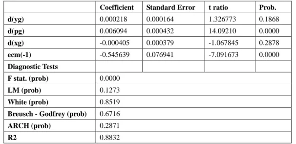
differences of the levels of gap variables obtained by using the Kalman Filter. Coefficient of the error correction term, on the other hand, represents the reaction of independent variables to deviations from the equilibrium. More clearly, the error correction coefficient gives information about the percentage of correction of the deviation from the equilibrium after a period of time (Dougherty, 2011). In practice, the error correction coefficient is expected to take a value between 0 and -1 and to be statistically significant. Statistical significance of the error correction term shows that there is a long-term causality among the variables. F statistic which indicates the significance of variables as a whole, gives information about short-term causality among variables. Estimation results of the error correction model and some diagnostic tests are given in Table 3.
Table 3. Estimation Results of Error Correction Model
Coefficient Standard Error t ratio Prob.
d(yg) 0.000218 0.000164 1.326773 0.1868 d(pg) 0.006094 0.000432 14.09210 0.0000 d(xg) -0.000405 0.000379 -1.067845 0.2878 ecm(-1) -0.545639 0.076941 -7.091673 0.0000 Diagnostic Tests F stat. (prob) 0.0000 LM (prob) 0.1273 White (prob) 0.8519
Breusch - Godfrey (prob) 0.6716
ARCH (prob) 0.2871
R2 0.8832
An examination of the table reveals that both the coefficient of the error correction term and the model as a whole are significant. This suggests the existence a short- and long-term causalities among the estimated gap variables. The coefficient value of the error correction term is interpreted as one unit of deviation from the equilibrium is corrected by 55% in the next period. In other words, it takes almost 6 months to reach the equilibrium again.
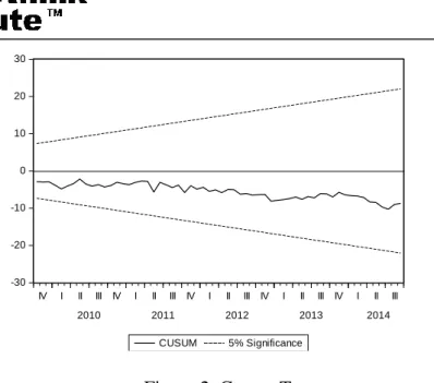
On the other hand, diagnostic tests of the model confirm that the estimated model is appropriate for accounting in explaining the relevant relationship discussed. The Cusum Test shown in the Figure 2 also shows that the estimated model has a stable structure.
-30 -20 -10 0 10 20 30
IV I II III IV I II III IV I II III IV I II III IV I II III
2010 2011 2012 2013 2014
CUSUM 5% Significance
Figure 2. Cusum Test
4. Conclusion
The natural rate of interest is considered the key variable to maintain the price stability and to converge production on the potential level. For this reason, central banks need natural rate of interest to identify the current stance of the monetary policy and to make suitable changes in policies. It is crucial, therefore, in conducting the monetary policy to estimate the natural rate of interest which is an unobservable variable and to identify its difference from the existing policy interest rate.
Although there are many studies in the literature intended to estimate the natural rate of interest, the number of studies conducted on Turkey is very limited. Therefore, in addition to determining the level of natural rate of interest, the current study examines the cointegration between the variables that affect this level and natural rate of interest. The Kalman filtering technique used in determination of the natural rate of interest allows it to be handled as a variable that takes values varying on the basis of the time rather than a constant value. The current natural rate of interest that is obtained is higher than the policy rate of interest but lower than the borrowing market rate of interest. This shows that the inflationary pressure has increased and there is a case of moving away from the inflation target in the direction of deviation from the top.
According to the estimated error correction model, the variables that have the most important effects on the natural rate of interest are the general price level and production volume. Deviations from the potential values of such variables are basic variables that determine the natural rate of interest. Depending on the decreasing pass through effect of the foreign exchange rate as a result of the floating exchange rate regime, deviations from the potential value observed in the foreign exchange rate have limited effect. The high speed of adjustment shows that markets react to the monetary policy in a short period of time and that a fast dynamic process is experienced in returning to the equilibrium process. The causality tests also yield results in support of this finding. Consequently, it is understood that the Central Bank should take realistic steps in conducting the monetary policy toward primarily the inflation target.
References
Adolfson, M. et al (2011). Optimal Monetary Policy in an Operational Medium-Sized DSGE Model. Journal of Money, Credit and Banking, 43(7), 1287-1331.
https://doi.org/10.1111/j.1538-4616.2011.00426.x
Basdenvant, O. et al (2004). Estimating a time varying neutral real interest rate for New
Zealand. Reserve Bank of New Zealand Discussion Paper Series DP 2004/01.
Bernhardsen, T., & Gerdrup, K. (2007). The Neutral Real Interest Rate. Norges Bank
Economic Bulletin, 2(7).
Bjorksten, N. & Karagedikli, O. (2003). Neutral Real Interest Rates Revisited. Reserve Bank
of New Zealand Bulletin, 66(3), 18-27.
Bomfim, A. (1997). The Equilibrium Fed Funds Rate and the Indicator Properties of Term Structure Spreads. Economic Inquiry, 35(4).
https://doi.org/10.1111/j.1465-7295.1997.tb01967.x
Calderon, C., & Gallego, F. (2002). La Tasa de Interés Real Neutral en Chile. Economía Chilena, 5(2), 65-72.
Castillo. P. et al (2006). Measuring the Natural Interest Rate for the Peruvian Economy, Working Paper 2006-003, Central Reserve Bank of Peru.
Chui, C. K., & Chan, G. (2009). Kalman Filtering with Real Time Applications. Berlin:Springer.
Cuaresma, J. et al (2003). Searching for the Natural Rate of Interest: A Euro-Area
Perspective. Austria National Bank Working Paper Series. 84.
Dougherty, C. (2011). Introduction to Econometrics (4th. Ed.).Londor: Oxford University Press
Duarte, J. (2010). Measuring the Natural Interest Rate in Brazil. Institute of Brazilian Business and Public Management Issues. Washington: George Washington University). ECB (2004). The Natural Real Interest Rate in the Euro Area. Monthly Bulletin. May. (Frankfurt: European Central Bank).
Fuentes, R., & Gredig, F. (2007). Estimating the Chilean Natural Rate of Interest. Working Paper No. 448 (Santiago: Central Bank of Chile).
Giammarioli, N. & Valla, N. (2003). The Natural Real Rate of Interest in the Euro Area. Working Paper Series 233, European Central Bank.
Gonzalez, A.et al (2012). Output Gap and Neutral Interest Rate Measures for Colombia. Working Paper No.726. Central Bank of Colombis.
Gonzalez, E. et al (2010). Estimations of the Natural Rate of Interest in Colombia. Working Paper No.626. Central Bank of Colombia.
Gujarati, D. N., & Porter, D. C. (2009). Basic Econometrics. (5th ed). New York: McGraw-Hill.
Hill, R. C. et al (2011). Principles of Econometrics. (4th ed) Hoboken, NJ: Wiley.
Humala, A., & Rodriguez, G. (2009). Estimation of a Time Varying Natural Interest Rate for
Peru. Working Paper 2009-009, Central Reserve Bank of Peru.
Lam, J. P., & Tkacz, G. (2004). Estimating Policy-Neutral Interest Rates for Canada Using a Dynamic Stochastic General Equilibrium Framework. Swiss Journal of Economics and
Statistics, 140(1), 89-126.
Laubach, T., & Williams, J.C. (2003). Measuring the Natural Rate. The Review of Economics
and Statistics, 85(4), 1063-1070. https://doi.org/10.1162/003465303772815934
Minella, A. et al (2002). Inflation Targeting in Brazil: Lessons and Challenges. Technical Report No. 53, Central Bank of Brazil.
Neiss, K., & Nelson, E. (2001). The Real Interest Rate Gap as an Inflation Indicator. Bank of England Working Papers 130.
Ogunc, F., & Batmaz, I. (2011). Estimating the Neutral Real Interest Rate in an Emerging Market Economy. Applied Economics, 43(3), 683-693.
https://doi.org/10.1080/00036840802599768
Pasricha, G. K. (2010). Kalman Filter and Its Economic Applications. MPRA Working Paper Series No.22734.
Pereda, J. (2010). Estimation of the Natural Interest Rate for Peru: A Financial Approach. Central Reserve Bank of Peru Working Paper 2010-018.
Perrelli, R. (2012). The Neutral Real Interest Rate in Brazil. International Monetary Fund Country Report No. 12/191.
Portugal, M., & Barcellos, P. C. (2009). The Natural Rate of Interest in Brazil between 1999 and 2005. RBE Rio De Janeiro, 63(2), 103-118.
Torres, J. L. (2007). La Estimacion de la Bracha del Product en Colombia. Central Bank of Colombia Discussion Paper No.462.
Woodford, M. (2002). Interest and Prices. (New York: Princeton University Press)
Zarchan, P. et al (2009). Fundemantal of Kalman Filtering: A Practical Approach. (3rd ed) Reston: American Institute of Aeronautics and Astronautics).
Copyright Disclaimer
Copyright for this article is retained by the author(s), with first publication rights granted to the journal.
This is an open-access article distributed under the terms and conditions of the Creative Commons Attribution license (http://creativecommons.org/licenses/by/3.0/).