Analytical Solutions of Nonlinear Klein-Gordon Equations Using Multistep Modified Reduced Differential Transform Method

ANALYTICAL SOLUTIONS OF NON-LINEAR KLEIN-GORDON

EQUATIONS USING MULTISTEP MODIFIED REDUCED

DIFFERENTIAL TRANSFORM METHOD

by

Che Haziqah CHE HUSSIN a,b*, Ahmad Izani MD. ISMAILa, Adem KILICMAN c,d,e, and Amirah AZMI a

a _{School of Mathematical Sciences, University Sains Malaysia, Gelugor, Penang, Malaysia} b _{Preparatory Centre of Science and Technology, University Malaysia Sabah, Jalan UMS,}

Sabah, Malaysia

c _{Department of Mathematics, Faculty of Science, Universiti Putra Malaysia, Selangor, Malaysia} d _{Institute for Mathematical Research, University Putra Malaysia, Selangor, Malaysia}

e _{Department of Electrical and Electronic Engineering, Istanbul Gelisim University,} Avcilar, Istanbul, Turkey

Original scientific paper https://doi.org/10.2298/TSCI181015045C

This paper explores the approximate analytical solution of non-linear Klein-Gor-don equations (NKGE) by using multistep modified reduced differential transform method (MMRDTM). Through this proposed strategy, the non-linear term is sub-stituted by associating Adomian polynomials obtained by utilization of a multistep approach. The NKGE solutions can be obtained with a reduced number of comput-ed terms. In addition, the approximate solutions converge rapidly in a wide time region. Three examples are provided to illustrate the effectiveness of the proposed method to obtain solutions for the NKGE. Graphical results are shown to represent the behavior of the solution so as to demonstrate the validity and accuracy of the MMRDTM.

Key words: Adomian polynomials, multistep approach, NKGE reduced differential transform method

Introduction

Klein-Gordon (KG) equation is an important equation which is related to the Schroedinger equation. It is applied widely in fields, such as quantum mechanics, solid state physics and non-linear optics [1]. The KG equation is one of the important equations in solitons studies, particularly in the examination of solitons interactions for a collisionless plasma and the recurrence of initial states [2, 3].

Many techniques have been implemented to derive the approximate analytical solu-tion of the KG equasolu-tions. In 2011, Servi and Oturanc [4] executed reduced differential trans-form method (RDTM) to solve KG equation. On the other hand, to calculate the exact traveling wave solutions to the KG equation, Hafez et al. [5] used the novel (G’/G)-expansion method. Meanwhile, Venkatesh, et. al, [6] used Lagendre wavelet-based approximations to solve KG equation that arise in quantum field theory using wavelets. Recently, Agom and

mi [7] proposed the modified Adomian decomposition method (ADM) to find the exact solution to NKGE with quadratic non-linearity.

Many PDE, ODE and delay differential equations have been solved by utilizing DTM and RDTM [8-14]. Ray [15] proposed an adjustment on the fractional RDTM and executed it to obtain solutions of fractional Korteweg de Vries (KdV) equations. Through this method-ology, the modification included the substitution of the non-linear term by relating Adomian polynomials. Therefore, the solutions of non-linear initial value problem can be obtained in an easier way with reduced computed terms. Further, El-Zahar [16] introduced adaptive multistep DTM to obtain solution of singular perturbation initial-value problems. It yields the solution in a rapid convergent series which results in the solution converging in wide time region. Recent-ly, Che Haziqah et. al. [17] has proposed and implemented MMRDTM for solving non-linear Schroedinger equations (NLSE). The results showed the approximate solutions of NLSE with high accuracy were obtained.

In this study, we combine modification in [15] and multistep approach in [16] to imple-ment a new technique called MMRDTM. The key benefit of the proposed technique is that it pro-duces an analytical approximation in a rapid convergent sequence with elegant computed terms.

Application of MMRDTM for the solution of NKGE

Let us use the general NKGE of the form [18]:

( , ), , 0

− + + k = ∈Ω < ≤

tt xx t

u αu βu γu f x t x t T (1)

which is subjected to the following initial conditions:

0 ( ,0)= ( ), ≤ ≤ u x u x a x b 1 ( ,0)= ( ), ≤ ≤ t u x u x a x b

where Ω =[ , ]a b ⊂R u x t, ( , ) denotes the wave displacement at position x and time t, u x0( )is

a known function and α β, , and γ are real numbers (γ ≠0). The k=2 is the case of quadratic non-linearity and k=3 for a cubic non-linearity.

Applying basic properties of modified RDTM to eq. (1), we obtain:

(

)(

)

2 2, ₂ , , , 0 1 ( ) ( ) ( , ) 2 1 + =   ∂ _{ }  =_{    }− − + _ + + ∂       

∑

n k i k i k i k i k U x U x A U f x t k k x γ β (2)

From the initial condition, we can write:

0( )= ( )

U x f x (3)

The non-linear term can be composed:

[

0 1

]

0 ( , ) _n ( ), ( ), , ( )_n n Nu x t ∞ A U x U x U x = =

∑

…

We acquire the following U x_k( ) values by straightforward iterative estimation and substituting eq. (3) into eq. (2). Then, inversely, the transformation of the set of values { ( )}U xk nk=₀

gives the n-terms estimation solution:

[ ]

0 ( , ) ( ) , 0, = =

∑

K k ∈ k k u x t U x t t T

For i=1,2, ,… M, the interval [0, ]T is separated into N subintervals [ , ]t ti−1 i by using equal step size of h T M= / and nodes t is_i = . Multistep RDTM is computed according to the following steps.

Firstly, the RDTM is applied to the initial value problem in interval [0, ].t1 From that

point, the estimated result is obtained using the initial conditions u x( ,0)= f x u x0( ), ( ,0) ( ).1 =f x1

[ ]

1 ,1 1 0 ( , ) ( ) , 0, = =

∑

K k ∈ k k u x t U x t t t

For i≥2, the initial conditions u x ti( , i−₁)=ui−₁(x t, i−₁), /

(

∂ ∂t u x t

)

i( ,i−₁) are utilized at

each subinterval [ , ],t ti−₁ i and the multistep RDTM is applied to the initial value problem in

1

[ , ],t ti− i where t0 is substituted by ti−1. For i=1,2, ,… M, the procedure is continued and

re-peatedly performed to obtain estimated solutions u x t_i( , ) in sequence form that is:

[

]

, 1 1 0 ( , ) ( )( − ) , −, = =

∑

K − k ∈ i k i i i i k u x t U x t t t t t

In fact, the MMRDTM expects the following solution:

1 1 2 1 2 1 ( , ) [0, ] ( , ) [ , ] ( , ) ( , ) [ − , ] ∈   _∈  =    _∈    M M M u x t t t u x t t t t u x t u x t t t t

We found that the calculation of MMRDTM is straightforward with better computa-tional performance for all values of .s If the step size h T= , we can easily notice that the MMRDTM reduces to the MRDTM

Numerical results and discussions

We give three test problems to evaluate if this method is efficient and accurate to solve NKGE.

Example 1. Consider the second-order NKGE [19]: 2 ₀

tt xx

u −u +u = (4)

with the following indicated initial condition:

( ,0) 1 sin( ) u x = + x 0 ( ,0) t x u =

There is no exact solution for this equation. Using basic properties of MMRDTM then followed by utilizing MMRDTM for eq. (4), we obtain the following equation:

(

)(

)

2 2, ₂ , , 0 1 ( ) ( ) 2 1 n k i k i k i k U x U x A k k x + =   ∂ _{ }  = _{+ +}   _{ }−  ∂        

∑

(5)

From the initial condition, we compose:

0( ) 1 sin( )

The following U x_k( ) values are obtained by substituting eq. (6) into eq. (5) by straightforward iterative calculation. Then, the inverse transformation of the set of values

6

6 0

{ ( )}U x k= gives the 6-terms estimated solution:

2 4

6

3 3 1

( , ) 1 sin( ) sin( ) cos(2 )

2 4 4

25_{sin( )} 1_{cos(2 )} 1 1 _{sin(3 )}

48 4 4 48

79 _{sin( )} 17 _{cos(2 )} 41 _{sin(3 )} 263 1 _{cos(4 )}

480 144 1440 2880 576   = + + −_ − + _ +     +_ − + − _ +     + −_ + + − − _   u x t x x x t x x x t x x x x t where t∈[0.1,0.3].

For i=1,2,3, the interval [0.1,0.3] is divided into 3 subintervals [ , ]t ti−1 i by equaliz-ing step size by usequaliz-ing the nodes t ih_i= . For i≥2, the initial conditions u x ti( ,i−1)=

(

)

(

)

1( , 1), / ( , 1) / 1( , 1)

− − − − −

=u_i x t_i ∂ ∂t u x t_{i i} = ∂ ∂t u_i x t_i will be used at each subinterval [ , ]t ti−1 i Then, the modified RDTM is utilized to the initial value problem in interval [ , ]t ti−1 i , where t0

is substituted by ti−1. The process is continuously and repeatedly performed to obtain estimated

solutions u x t i_i( , ), =1,2,3 for the solution u x t( , ), such as:

, 1 1 0 ( , ) ( )( − ) , [ , ]− = =

∑

K − k ∈ i k i i i i k u x t U x t t t t t

We compare the approximate results with DTM and RDTM. It is clear that the MMRDTM result converges for x=0 until x=1 compared with the DTM results obtained by Kanth and Aruna [19]. From the results, figs. 1(a) and 1(b) show approximation of MMRDTM and RDTM for t∈[0,1] and x∈ −[ 4,4], respectively. The performance error analyses obtained by MMRDTM are tabulated in tab. 1.

U(x) U(x) x (a) MMRDTM RDTM (b) t x t

Figure 1. Approximation result of MMRDTM and RDTM for Example 1

(for color image see journal web site)

Example 2. Consider the second-order non-linear Klein Gordon [17]:

( )

( )

2 _cos 2_cos2

− + = − +

tt xx

u u u x t x t (7)

which is subjected to the initial condition:

( )

,0 =

u x x

( )

,0 =0 t

The exact solution of this equation is xcos( )t .

Using basic properties of MMRDTM and then applying MMRDTM to eq. (7), we obtain:

Table 1. Results of MMRDTM and RDTM approximate solutions for Example 1

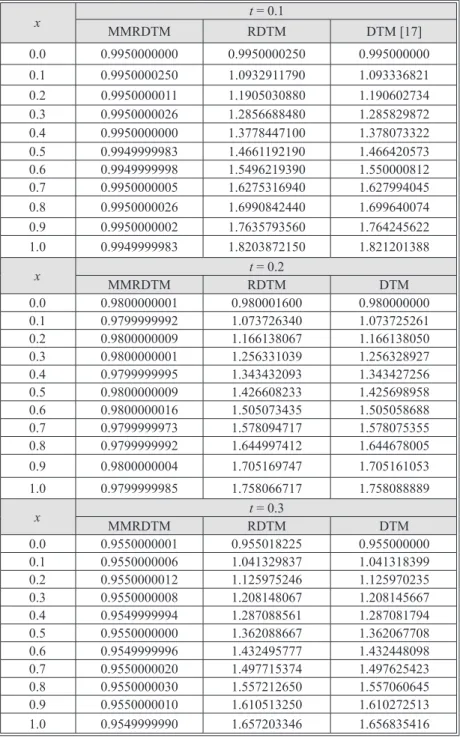
x _{MMRDTM RDTM}t = 0.1 _{DTM [17]} 0.0 0.9950000000 0.9950000250 0.995000000 0.1 0.9950000250 1.0932911790 1.093336821 0.2 0.9950000011 1.1905030880 1.190602734 0.3 0.9950000026 1.2856688480 1.285829872 0.4 0.9950000000 1.3778447100 1.378073322 0.5 0.9949999983 1.4661192190 1.466420573 0.6 0.9949999998 1.5496219390 1.550000812 0.7 0.9950000005 1.6275316940 1.627994045 0.8 0.9950000026 1.6990842440 1.699640074 0.9 0.9950000002 1.7635793560 1.764245622 1.0 0.9949999983 1.8203872150 1.821201388 x _{MMRDTM RDTM}t = 0.2 _DTM 0.0 0.9800000001 0.980001600 0.980000000 0.1 0.9799999992 1.073726340 1.073725261 0.2 0.9800000009 1.166138067 1.166138050 0.3 0.9800000001 1.256331039 1.256328927 0.4 0.9799999995 1.343432093 1.343427256 0.5 0.9800000009 1.426608233 1.425698958 0.6 0.9800000016 1.505073435 1.505058688 0.7 0.9799999973 1.578094717 1.578075355 0.8 0.9799999992 1.644997412 1.644678005 0.9 0.9800000004 1.705169747 1.705161053 1.0 0.9799999985 1.758066717 1.758088889 x _{MMRDTM RDTM}t = 0.3 _DTM 0.0 0.9550000001 0.955018225 0.955000000 0.1 0.9550000006 1.041329837 1.041318399 0.2 0.9550000012 1.125975246 1.125970235 0.3 0.9550000008 1.208148067 1.208145667 0.4 0.9549999994 1.287088561 1.287081794 0.5 0.9550000000 1.362088667 1.362067708 0.6 0.9549999996 1.432495777 1.432448098 0.7 0.9550000020 1.497715374 1.497625423 0.8 0.9550000030 1.557212650 1.557060645 0.9 0.9550000010 1.610513250 1.610272513 1.0 0.9549999990 1.657203346 1.656835416

( ) ( )( )

2 2 2 2, 2 , , 0 1 _{( ) cos cos} 2 1 ! 2 ! 2 + =   ∂ _{ } π  π  =_{ + +}  _∂  − − _ _+ _ __     

∑

n k i k i k i k x k x k U x U x A k k x k k (8)

From the initial condition, we write:

0( ) =

U x x (9)

The U xk( ) values is obtained by substituting eq. (9) into eq. (8) by straightforward

iterative calculation. Then, the inverse transformation of the set of values 6

6 0

{ ( )}U x k= gives the

6-terms approximation solution:

( )

[ ]

2 2 4 2 2 6 1 1 1 , x 2 8 24 1 1 1 1 1 _{1 , 0,1} 120 15 8 24 144 720   = − +_ + _ +       +_ − _ + _− − _ ∈     u x t x t x x t x x x x x t t

Divide the interval [0,1] into 10 subintervals [ , ],t t ii−₁ i =1,2, ,10, … by using equal

step size h=0.1 and the nodes t ih_i= . The core ideas of the MMRDTM are as follows. Firstly, the RDTM is applied to the initial value problem over the interval [0, ].t₁

For i≥2, we use the initial conditions u x ti( , i−₁)=ui−₁(x t, i−₁ ,)

(

∂ ∂/ t u x t

)

i( , i−₁)=

(

/

)

−1( , −1)

= ∂ ∂t u_i x t_i at each subinterval [ , ],t ti−₁ i and the MRDTM is applied to the initial value problem over the interval [ , ],t ti−₁ i where t0 is replaced by ti−1. Next, the multistep scheme for

repeating process are u x( ,0)= f x u x₀( ), ( ,0) 0.₁ = The process is continued and repeated to generate a sequence of approximate solutions u_i( , ),x t i=1, , ,10,2… for the solution u x t( , )

such as: , 1 1 0 ( , ) ( )( −) , [ , ]− = =

∑

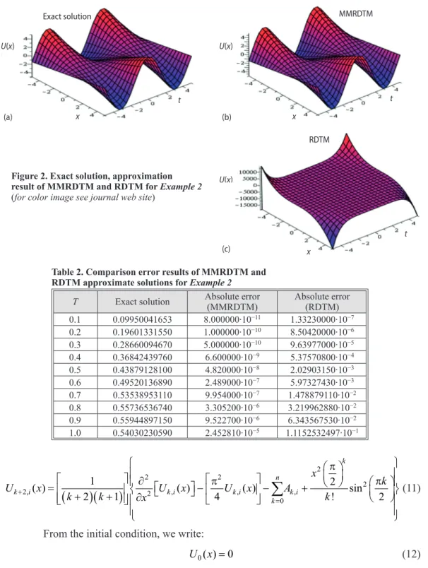
K − k ∈ i k i i i i k u x t U x t t t t t

Figure 2(a) shows the exact solution, fig. 2(b) shows the graph of approximate solu-tion MMRDTM for t ∈ [–5,5] and x ∈ [–5,5] while fig. 2(c) shows the graph of approximate solution RDTM for t ∈ [–5,5] and x ∈ [–5,5]. Obviously, the multistep approximate solutions for this type of NKGE are very close to the exact solutions. The performance error analyses obtained by MMRDTM are summarized in tab. 2.

Example 3. Consider the second-order NKGE [17]: 2 2 2_sin2 4 2 π π  − + + = _{ }   tt xx u u u u x t (10)

subject to the initial condition:

( ,0) 0= u x ( ,0) 2 π = t u x x

The exact solution of this equation is xsin( /2)πt .

Using fundamental properties of MMRDTM then utilizing MMRDTM to eq. (10), we can get:

(

)(

)

2 2 2 2 2, 2 , , , 0 1 2 ( ) ( ) ( ) sin 2 1 4 ! 2 + =  _{ π}   _{ }   ∂ _{ } π    π  =_{    }−_{ }− + _{ } + + ∂             

∑

k n k i k i k i k i k x _k U x U x U x A k k x k (11)

From the initial condition, we write:

0

( ) 0=

U x (12)

Separate the interval [0,1] into 10 subintervals [ , ],t t ii−1 i =1,2, ,10, … of equal step size h=0.1 and use the nodes t ih_i= . The main ideas of the MMRDTM are as follows. Firstly, the RDTM is applied to the initial value problem over the interval [0, ].t1

Table 2. Comparison error results of MMRDTM and RDTM approximate solutions for Example 2

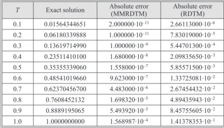
T Exact solution Absolute error_(MMRDTM) Absolute error_(RDTM) 0.1 0.09950041653 8.000000∙10−11 _{1.33230000∙10}−7 0.2 0.19601331550 1.000000∙10−10 _{8.50420000∙10}−6 0.3 0.28660094670 5.000000∙10−10 _{9.63977000∙10}−5 0.4 0.36842439760 6.600000∙10−9 _{5.37570800∙10}−4 0.5 0.43879128100 4.820000∙10−8 _{2.02903150∙10}−3 0.6 0.49520136890 2.489000∙10−7 _{5.97327430∙10}−3 0.7 0.53538953110 9.954000∙10−7 _{1.478879110∙10}−2 0.8 0.55736536740 3.305200∙10−6 _{3.219962880∙10}−2 0.9 0.55944897150 9.522700∙10−6 _{6.343567530∙10}−2 1.0 0.54030230590 2.452810∙10−5 _{1.1152532497∙10}−1

Figure 2. Exact solution, approximation result of MMRDTM and RDTM for Example 2

(for color image see journal web site)

U(x) x (b) U(x) (c) t x t MMRDTM U(x) x (a) t RDTM Exact solution

Figure 3(a) shows the exact solution, fig. 3(b) illustrates the graph of approximate solution MMRDTM for t ∈ [–5, 5] and x ∈ [–5, 5] while fig. 3(c) illustrates the graph of ap-proximate solution RDTM for t ∈ [–5, 5] and x ∈ [–5, 5]. Therefore, as we can see the multistep approximate solutions for this type of NKGE are very close to the exact solutions. The perfor-mance error analyses obtained by MMRDTM are summarized in tab. 3.

Table 3. Comparison error results of MMRDTM and RDTM approximate solutions for Example 3

T Exact solution Absolute error_(MMRDTM) Absolute error_(RDTM) 0.1 0.01564344651 2.000000∙10–11 _{2.66113000∙10}–6 0.2 0.06180339888 1.000000∙10–11 _{7.83019000∙10}–5 0.3 0.13619714990 1.000000∙10–9 _{5.44701300∙10}–4 0.4 0.23511410100 1.680000∙10–8 _{2.09835650∙10}–3 0.5 0.35355339060 1.558000∙10–7 _{5.85571500∙10}–3 0.6 0.48541019660 9.623000∙10–7 _{1.33725081∙10}–2 0.7 0.62370456700 4.483000∙10–6 _{2.67454432∙10}–2 0.8 0.7608452132 1.698320∙10–5 _{4.89435943∙10}–2 0.9 0.8889195065 5.493920∙10–5 _{8.45755605∙10}–2 1.0 1.0000000000 1.568987∙10–4 _{1.41378353∙10}–1

Figure 3. Exact solution, approximation result of MMRDTM and RDTM for

Example 3 (for color image see journal web site) U(x) x (a) t Exact solution U(x) x (b) t MMRDTM U(x) (c) x t RDTM

Conclusion

In this paper, we proposed and applied an approximate analytical method which is called the MMRDTM to solve the 1-D NKGE. In this new strategy, the modification involves the replacement of non-linear term by its Adomian polynomials and a multistep approach. The results demonstrate that the approximate solutions of NKGE have high precision. In conclu-sion, we can state that the MMRDTM is a valid and efficient method for finding analytic ap-proximate solution for these types of equations. The computations in this paper were obtained by utilizing MAPLE 13.

Acknowledgment

The authors express their appreciation to Malaysian Ministry of Higher Education and Universiti Malaysia Sabah for supporting this research. We also have financial support from Universiti Sains Malaysia research grant 304/PMATHs/6315088.

References

[1] Wazwaz, A.,The Modified Decomposition Method for Analytic Treatment of Differential Equations, 17 (2006b), 3, pp. 165-176

[2] El-Sayed, S. M., The Decomposition Method for Studying the Klein-Gordon Equation, Chaos, Solitons

and Fractals, 18 (2003), 5, pp. 1025-1030

[3] Wazwaz, A., Compactons, Solitons and Periodic Solutions for Some Forms of Nonlinear Klein-Gordon Equations, Chaos, Solitons and Fractals, 28 (2006a), 4, pp. 1005-1013

[4] Servi, S., Oturanc, G., Reduced Differential Transform Method for Solving Klein-Gordon Equations,

Proceedings, World Congress on Engineering, London, 2011,Vol. I, pp. 2-6

[5] Hafez, M. G., et al., Exact Traveling Wave Solutions to the Klein-Gordon Equation using the Novel (G’/G)-Expansion Method, Results In Physics, 4 (2014), C, pp. 177-184

[6] Venkatesh, S. G., et al., An Efficient Approach for Solving Klein-Gordon Equation Arising in Quantum Field Theory using Wavelets, Computational and Applied Mathematics, 37 (2016), 1, pp. 81-98

[7] Agom, E. U., Ogunfiditimi, F. O., Exact Solution of Nonlinear Klein-Gordon Equations with Quadratic Nonlinearity by Modified Adomian Decomposition Method, Journal of Mathematical Computational

Sci-ence, 8 (2018), 4, pp. 484-493

[8] Jameel, A. F., et al., Differential Transformation Method for Solving High Order Fuzzy Initial Value Prob-lems, Italian Journal of Pure and Applied Mathematics, 39 (2018), Mar., pp. 194-208

[9] Rao, T. R. R., Numerical Solution of Sine Gordon Equations through Reduced Differential Transform Method, Global Journal of Pure and Applied Mathematics, 13 (2017), 7, pp. 3879-3888

[10] Acan, O., Keskin, Y., Reduced Differential Transform Method for (2+1) Dimensional Type of the Zakharov-Kuznetsov ZK (n, n) Equations, AIP Conference Proceedings, 1648 (2015), 1, 370015 [11] Marasi, H. R., et al., Modified Differential Transform Method for Singular Lane-Emden Equations in

Integer and Fractional Order, Journal of Applied and Engineering Mathematics, 5 (2015), 1, pp. 124-131 [12] Benhammouda, B., Leal, H. V., A New Multi-Step Technique with Differential Transform Method for

Analytical Solution of Some Nonlinear Variable Delay Differential Equations, SpringerPlus, 5 (2016), 1723

[13] Kang-Le, W., Kang-Jia W., A Modification of the Reduced Differential Transform Method for Fractional Calculus, Thermal Science, 22 (2018), 4, pp. 1871-1875

[14] Hossein, J., et al., Reduced Differential Transform and Variational Iteration Methods for 3-D Diffusion Model in Fractal Heat Transfer Within Local Fractional Operators, Thermal Science, 22 (2018), Suppl. 1, pp. S301-S307

[15] Ray, S. S. ,Numerical Solutions and Solitary Wave Solutions of Fractional KdV Equations using Modified Fractional Reduced Differential Transform Method, Journal of Mathematical Chemistry, 51 (2013), 8, pp. 2214-2229

[16] El-Zahar, E. R., Applications of Adaptive Multi Step Differential Transform Method to Singular Pertur-bation Problems Arising in Science and Engineering, Applied Mathematics and Information Sciences, 9 (2015), 1, pp. 223-232

[17] Che Haziqah C. H., et al., Analytical Solutions of Nonlinear Schrodinger Equations using Multi-step Modified Reduced Differential Transform Method, International Journal of Advanced Computer

Tech-nology, 7 (2018), 11, pp. 2939-2944

[18] Huang, D., et al., Numerical Approximation of Nonlinear Klein-Gordon Equation Using an Element-Free Approach, Mathematical Problems in Engineering, 2015 (2015), ID 548905

[19] Kanth, A. S. V. R., Aruna, K., Differential Transform Method for Solving the Linear and Nonlinear Klein-Gordon Equation, Computer Physics Communications, 180 (2009), 5, pp. 708-711

Paper submitted: October 15, 2018 Paper revised: November 12, 2018 Paper accepted: January 16, 2019

© 2019 Society of Thermal Engineers of Serbia Published by the Vinča Institute of Nuclear Sciences, Belgrade, Serbia. This is an open access article distributed under the CC BY-NC-ND 4.0 terms and conditions