Human motion analysis and action recognition

(1)

T.C.

BAHÇEŞEHİR ÜNİVERSİTESİ

HUMAN MOTION ANALYSIS AND ACTION

RECOGNITION

Master Thesis

(2)

T.C.

BAHÇEŞEHİR ÜNİVERSİTESİ

Institute of Science

Computer Engineering Graduate Program

HUMAN MOTION ANALYSIS AND ACTION

RECOGNITION

Master Thesis

Murat NURULLAHOĞLU

Supervisor: ASSC. PROF.DR. ADEM KARAHOCA

(3)

T.C

BAHÇEŞEHİR ÜNİVERSİTESİ

Graduate School in Sciences Computer Engineering Graduate Program

Name of the thesis: HUMAN MOTION ANALYSIS AND ACTION RECOGNITION Name/Last Name of the Student: Murat Nurullahoğlu

Date of Thesis Defense:

The thesis has been approved by the Institute of Graduate School in Sciences. Prof. Dr. Erol Sezer

Director

Signature

I certify that this thesis meets all the requirements as a thesis for the degree of Master of Science.

Assc. Prof. Dr. Adem Karahoca Program Coordinator

Signature

This is to certify that we have read this thesis and that we find it fully adequate in scope, quality and content, as a thesis for the degree of Master of Science.

Examining Committee Members Signature

Title Name and Surname

Thesis Supervisor Assc.Prof.Dr. Adem Karahoca

Member Prof.Dr. Nizamettin Aydın

(4)

ACKNOWLEDGEMENTS

It is a pleasure to thank the many people who made this thesis possible, first and foremost, I would like to thank my mother, father, sister who have untiringly shown me guidance, patience and love. Without them, I never would have been able to get here.

I would like to express my deep gratitude both personally and professionally, to my advisor, Assc. Prof. Adem Karahoca, without whose guidance and encouragement the completion of this study would be impossible. I will remember every word of his valuable advice in my future studies.

I would also thank to the committee members. I would also like to express my thanks to the committee members Prof. Nizamettin Aydın and Asst. Prof. Dr. M. Alper Tunga for carefully reading the thesis manuscript and their valuable suggestions.

I would like to thank CSE faculty and research assistants for making my two years at Bahçeşehir University a great experience.

Finally, I would like to thank all my friends for their motivation.

(5)

ABSTRACT

HUMAN MOTION ANALYSIS AND ACTION RECOGNITION

Nurullahoğlu Murat

The Institute of Sciences, Computer Engineering Graduate Program

Supervisor: Assc. Prof.Dr. Adem Karahoca

August 2008, 62 pages

The goal of human activity recognition systems is to build a system that can automatically infer a range of predefined activities, such as running, handclapping, etc, from recorded video sequences. Such a computerized system would be of great use for a variety of applications ranging from video surveillance for security to human-machine interaction. Typically, pattern recognition is the key component of such a system, where the goal is to classify, or more specifically “recognize” the data, based on a priori knowledge or statistical information extracted from the patterns.

In this study, we presented a comparison of several well-known pattern recognition techniques for a human activity recognition system. Firstly, the database of short video sequences that each consisting of a set of predefined actions, i.e. running, jogging, boxing and handclapping, performed by different people at different environments are used. Then, using sophisticated image processing and computer vision algorithms, the segmentation of the human performing the action was achieved and a set of descriptive features were extracted for each activity performed. Motion History Images (MHI) were used to describe these activities in a qualitative way and computed Hu moments, a widely used and well-known feature set to describe 2D or 3D shapes, for further processing. Several feature extraction and classification methods are compared using different combinations and the results are analyzed. These methods are Principle Component Analysis and Linear Discriminant Analysis.

The features with Support Vector Machines and K Nearest Neighbours classifiers are tested. The best results are taken in Hu moments for KNN classifier, K=1 and PCA for KNN. The both accuracy is 95 percent. The worst results are taken in PCA for SVM. The accuracy is 80.6 percent.

(6)

ÖZET

INSAN HAREKETI ANALIZI VE HAREKET TANINMASI

Nurullahoğlu, Murat

Fenn Bilimleri Enstitüsi, Bilgisayar Mühendisliği Yüksek Lisan Programı

Danışman: Doç.Dr. Adem Karahoca

Ağustos 2008, 62 sayfa

İnsan hareketi tanıma sistemlerinin ana amacı, önceden tanımlanmış koşma, el çırpma gibi hareketleri otomatik olarak tanınmasını sağlamaktır. Güvenlik için izlemeden, insan-makine etkileşimine kadar geniş bir yelpazede bu sistemler kullanılmaktadır. Bu sistemleri en önemli birimi örüntü tanıma işlemleridir.

Bu çalışmada, insan hareketlerinin tanınması için, iyi bilinen birkaç tanıma algoritması karşılaştırılmıştır. Öncelikle, önceden tanımlanmış olan ve farklı insanlar tarafından gerçekleştirilen koşma, jogging, el çırpma ve boks yapma gibi hareketlerden bir veritabanı oluşturulmuştur. Bu hareketlerin hepsi için geçmis hareket imgelerinden Hu moment’leri hesaplanmıştır ve birkaç özellik çıkarma algoritması ve tanıma algoritmalarıyla farklı kombinasyonlar kullanılarak test edilip sonuçları analiz edilmiştir.

Test etmek için Support Vector Machines (SVMs) ve K Nearest Neighbours (KNN) algoritmaları kullanılmıştır. En iyi sonucu, Hu moment ve PCA ile elde edilen özelliklerin KNN ile testi sonucunu yüzde 95 başarı ile bulunmuştur. En kötü sonucu ise PCA ile oluşturulan özelliklerin SVMs ile test edilmesinde yüzde 80.6 ile elde edilmiştir.

Anahtarlar Kelimeler: Human activity recognition, motion history images (MHI), Hu moments, principal components analysis (PCA), linear discriminant analysis (LDA)

(7)

LIST OF TABLES

Table 4. 1 : The result of KNN classifier for each motion classes ... 41

Table 4. 2 : The result of SVM classifier for each motion classes ... 42

Table 4. 3 : Variance explained for all principal components... 44

Table 4. 4: The result of KNN classifier for each motion classes ... 47

Table 4. 6 : The result of KNN classifier for each motion classes ... 51

(9)

LIST OF FIGURES

Figure 3. 1 : Running man... 12

Figure 3. 2 : Mhi of running man ... 13

Figure 3. 3 : Orginal frame... 14

Figure 3. 4 : Background subtraction ... 14

Figure 3. 5 : After removing noisy pixels ... 15

Figure 3. 6 : Running man... 17

Figure 3. 8 : Handclapping man ... 17

Figure 3. 9 : Mhi of handclapping man ... 17

Figure 3. 10 : Class separation ... 27

Figure 3. 11 : Maximum-margin hyper planes for a SVM ... 34

Figure 4. 1 : Mhi of boxing man ... 38

Figure 4. 2 : Mhi of handclapping man ... 39

Figure 4. 3 : Mhi of jogging man ... 39

Figure 4. 5 : ROC Curve for each classes with KNN classifier ... 41

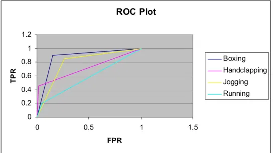
Figure 4. 6 : ROC Curve for each classes with SVM classifier ... 43

Figure 4. 7 : An example to explain and illustrate the theory of 2D PCA... 45

Figure 4. 8 : Zoom of the small area, where the samples of jogging... 46

Figure 4. 9 : ROC Curve for each classes with KNN classifier ... 47

(10)

Figure 4. 13 : ROC Curve for each classes with SVM classifier ... 53 Figure 4. 14 : ROC Curve for each classifier methods and their features ... 54

(11)

LIST OF SYMBOLS/ABBREVIATIONS

Hidden Markov Model : HHM K-Nearest Neighbours : KNN Linear Discriminant Analysis : LDA

Motion History Images : MHI

Principal Components Analysis : PCA

(12)

1. INTRODUCTION

Human Activity Recognition is to characterize the behaviour of a person. The ability of recognizing human and activities is a key importance to design a machine capable of interacting intelligently with a human-inhabited environment. Human Activity Recognition is used in many applications like security surveillance, medical diagnosis, choreography of dance and ballet, sign language translation, sports analysis and smart rooms (Gavrila & Davis 1996).

Event detection and human action recognition have gained more interest, among video processing community because they find various applications in automatic surveillance, monitoring systems (Liu & Chellappa (2007), Tan et al (2005), Venkatesh & Ramakrishnan (2004)). Video indexing and retrieval, robot motion, human–computer interaction and segmentation, and human motion analysis related issues studied from (Hernández et al. (2007), Han et al. (2007), Starner and Pentland (1995), Shavit and Jepson (1993)). Human motion analysis based on computer vision techniques has gained much attention to the modern researchers for its various practical applications. There are two fundamental questions in these applications. The first one is that how are things (pixels or cameras) moving? , the second one is “What is happening?”(Czyz and Liao (2006), Cao et al. (2004), Campbell et al. (2004), Bobick (1995), Lai et al. (2006)).

Principal Component Analysis (PCA) and Linear Discriminant Analysis (LDA) are both well-known techniques for feature extraction or sometimes referred to as dimensionality reduction. (Urtasun et al. (2006), Ormoneit et al. (2005)) used PCA in human motion analysis. PCA provides a compact representation by projecting the data onto a feature space that captures the most representative features. In the new feature space, the first principal component is associated with the largest eigen values of the covariance matrix that corresponds to the direction where data have the largest variance (Smith 2002). Dick and Brooks (2003) used LDA in their human motion analysis work. LDA requires

(13)

lower dimensional subspace that best discriminates data. Hu moments are statistical description of images using moment-based features, which have reasonable shape discrimination in a translation- and scale-invariant manner (Hu 1962).

Various approaches have been proposed for human motion analysis. We divided the prior work into three main classes. These are generic model recovery (model based),

appearance-based models, and direct motion-based recognition. The approach of the

generic model recovery is to recover the pose of the person or object at each time instant using a three-dimensional model. The main advantage of model based approach is evidence gathering techniques used the whole image sequence before making a choice on the model fitting. On the other hand, the computational costs, due to the complex matching and searching are the disadvantage of implementing a model based approach. The disadvantage of implementing a model based approach is that the computational costs, due to the complex matching and searching that has to be performed are high (Dawson 2002). Because of the fact that increasing computing power, this can be seen as less of a disadvantages especially in non real-time applications and most algorithmic implementations help to reduce this costs.

Another model of human analysis is the appearance-based models. The approach of this model is to use only the two dimensional appearance of the action of two-dimensional static used in a multitude of frameworks where a human action is seen by consecutive images of two-dimensional instances/poses of the object. The major advantage of using appearance based methods is the simplicity of parameter computation. However, the matching may not be one-to-one, and the losing of precise spatial information is the main disadvantage of the appearance-based models (Du & Charbon 2007)

The last model is the direct motion-based recognition model. The approach of this model is to characterize the motion itself without reference to the underlying static poses of the body. The main advantage of this approach is the lower computation complexity and simpler implementation and also it doesn’t require explicit feature and it

(14)

explicit geometric information, the trajectory-to-trajectory approach better determines large spatial temporal misalignments, can align video sequences acquired by different sensors and is less affected by changes in background (Rao et al. 2003).

This thesis presents an appearance-based approach to the recognition of human movement. In this study, main objective is to benchmarking the different combinations of feature extraction and classification algorithms and compare and discuss the outcomes. We used Principal Components Analysis (PCA) and Linear Discriminant Analysis (LDA) algorithms as feature extractors to better represent the feature space by reducing the dimensionality. We made tests on the resulting feature spaces using a number of classifiers such as K-Nearest Neighbours (KNN) and Support Vector Machines (SVM) with a linear kernel.

The thesis is organized as follows. Section 2 reviews related work on human motion recognition. Section 3 presents our methods for pre-processing and classification. Section 4 reports the detailed results using the classification algorithms with different classifier. Finally, conclusions are drawn in Section 5.

(15)

2. LITERATURE REVIEW

The number of approaches to recognizing motion, particularly human movement, has recently grown at a tremendous rate. As mentioned earlier, prior works can be categorized into three categories.

A. Generic model recovery, B. Appearance-based models, C. Direct motion-based recognition.

2.1 GENERIC HUMAN MODEL RECOVERY

One of the most common techniques to attain the three dimensional movement information is to recover the pose of the person or object at each time instant using a three-dimensional model. The model proposed is driven by attempting to minimize a residual measure between the projected models and object contours (e.g., edges of body in the image). The strong segmentation of foreground/background and also of the individual body parts are required to help the model organized process. Extending to the blurred sequence for these techniques is so difficult (Bobick & James 2001).

Wagg (2006) used model-based approach to automated extraction of walking people from video data, under indoor and outdoor capture conditions. He thought about Generalized Expectation-Maximization algorithm with the same solution approach. He used similar algorithm for local and global modelling strategies employed in a recursive process. Human shape and gait motion was used for extracting process. The extracted shape and motion information is applied to construct a gait signature and it is enough for recognition purposes.

Dawson’s (2002) work is related with semi-automatic gait recognition using model based approach. The spatial and temporal metrics extracted from the model. Such that

(16)

people walking pattern’s amplitude and variation in angles of the limp and transformed in eigenspace and he used Principle Component Analysis.

Rehg, Kanade (1995) described to the local tracking of articulated objects using a layered template representation of self-occlusions. Their approach is based on a kinematical model. This model was used to order the templates by their visibility to the camera. The effects of occlusion were captured to each template by attaching window functions. The experimental results are presented for 3D hand tracking under a significant amount of self-occlusion.

Goncalves (1995) presented a promoted 3D tracking of the human arm against a uniform background using a two cone arm model and a single camera. Their approach was about addressing the problem which estimated the human position and a human arm’s motion using its behaviour. The modelled arm was two truncated right-circular cones connected using spherical joints. The using recursive estimator for arm position was proposed. So the estimator with error signals obtained by comparing the projected estimated arm position with that of the actual arm in the image is provided. The system is tested on a real image sequence.

Rohr (1994) extended their approach to the whole body as claimed. He used a full-body cylindrical model for tracking walking humans in natural scenes. The model-based approach for the recognition of pedestrians was introduced. They represent the human body by 3D-Model consisting cylinder. They use data from medical motion studies for modelling the movement of walking. Kalman filter was applied the estimation of model parameters in consecutive images. Single number was given all the poses of a walking action.

Gavrila and Davis (1996) extended this work to a full-body model for tracking human motion against a complex background. Their approach is about dividing humans and recognizing their activities to two major components;

(17)

1 - Body poses recovery and tracking 2 - Recognition of movement patterns

They present a vision system for the 3D model-based tracking of unconstrained human movement. They used image sequences acquired simultaneously from multiple views. The decomposition approach and best search technique for the high dimensional pose parameter space was used. They recover the 3D body pose at each time instant without the use of markers.

2.1.1 Three-Dimensional Movement Recognition

Bottino at al. (2007) approach is based on 3D motion data. The motion captured in 3D by means of a model-based technique was divided into sequences. Each sequence was classified into one of the recognizable a classes using PCA based method

Campbell and Bobick (1995) used three-dimensional data of human body for commercially system. Their approach is about identifying sets of constraints of movement expressed using body-centered coordinates such as joint angles and in force only during a particular movement. Their techniques were developed using defined by space curves for a representation of movements. There were axes of joint angles and torso location and attitude in the phase space. Their system used this representation for recognizing movements in unsegmented data.

Siskind’s (1995) approach is like known object configurations. The input of his system developed consisted of line-drawings of a person, table, and ball. The moving object’s positions, orientations, shapes, and sizes are known at all times. The approach uses support, contact, and attachment primitives and event logic to determine the actions of dropping, throwing, picking up, and putting down. The problem of recognizing actions were addressed by this approach when the precise configuration of the person and environment is known while the methods from the previous section concentrate on the

(18)

2.2 APPEARANCE-BASED MODELS

"View-based Approach" is an addition to three - dimensional recognition approach. When an human setting out is seen by consecutive images of two-dimentional instances of the object, view-based approach attempts to use only the two dimensional appearance of the action of two-dimensional static used in a multitude of frameworks. In many methods, the normalized image of the object is necessary.

Silhouette techniques using multiple cameras and shape are used by Weinland at al. (2006) and new motion descriptors are presented. Motion history volumes which fuse action cues, as seen from different viewpoints and over short time periods, into a single three-dimensional representation sets up the main idea of these new motion descriptors.

Spatial-temporal templates are used by Dimitrijevic at al. (2006). The templates that they used represent the specific part on the walking cycle where the angle between the legs is greatest and the feet are on the ground. Six different camera views, excluding frontal and back view and different scales are covered by the templates.

Hand shapes commonly found in the American Sign Language that are image-based were worked by Rupe (2005). Describing the shape of the hand for region-based shape descriptor is completed by the generic Fourier descriptor as the single camera was for recognizing the hand shape. For recognition of the hand shapes Multi-class Support Vector Machine was used and to extract the arm from hand region before feature extracting he developed the wrist detection algorithm.

For object tracking and pose estimation, two different algorithms are used by Pradit Mittrapiyanuruk (2004). Two instances in a pair of images and performs 3D reconstruction followed by 3D pose estimation was the first method's principal part. An extension of the original Active Appearance Models takes part of the second method's matching algorithm. The principal of this extension is without any restriction on its geometry its allowing for the estimation of the 3D pose of any object.

(19)

Shape analysis and tracking are used by Hariataoglu at al. (2006). As for ordering the body parts on the silhouette boundary, shape analysis and tracking were used to construct models of people appearance.

For representation the action, action mostly hand motion in the actual greyscale images without background is used by Cui et al. (1995) and, Wilson and Bobick (1995). Due to obvious natural variations and different clothing, actions that include the appearance of the total body are not as visually consistent across different people as the hand looks are still rather similar over a wide range of people except the skin colour.

Cui’s approach is a spatiotemporal event included two kinds of information, the object of interest and the movement of the object. The movement of the object was divided into two components: global and local motions. The global motion captured gross motion in terms of position and also the local motion represented deformation, orientation and gesture changes.

The approach of Wilson and Bobick (1995) is to allow for multiple models. The model is about a systematic way for describing a set of existing sensor data and a method for measuring how well it described new sensor data. The approach is based on multiple models simultaneously, where the type of models might be quite distinct. To characterize images in an image sequence was used eigenvector decomposition of sets of images, orientation histograms, peak temporal frequencies, tracked position of objects in the frame, and optic flow field summaries. In addition to this, Hidden Markov Model (HHM) algorithm was used for recognition motion.

Yamato et al. (1992) searched body silhouettes, and Akita (1984) employed body contours/edges, As opposed to using the actual raw greyscale image. The feature of image sequence of Yamato is based on bottom up approach with HHM. Silhouettes of human actions in a Hidden Markov Model (HMM) where silhouettes of background-subtracted images are vector quantized and used as input to the HMMs were used.

(20)

In Akita's work (1984), the use of edges and some simple two-dimensional body configuration knowledge (e.g., the arm is a protrusion out from the torso) are used to determine the body parts in a hierarchical manner (first, find legs, then head, arms, trunk) based on stability. The chaining local contour information found Individual parts. Although these two approaches decreased some of the variability between people, some problems seemed, such as the disappearance of movement that happens to be within the silhouetted region and also the varying amount of contour/edge information that arises when the background or clothing is high versus low frequency (as in most natural scenes). Also, the problem of examining the entire body, as opposed to only the desired regions, still exists, as it does in much of the three dimensional work.

(21)

2.3 MOTION-BASED RECOGNITION

Direct motion recognition (Dait & Qiant 2004; Dawson 2002) is another approach for recognition motion. This approach is to characterize the motion itself without using body’s static poses. Both single “blob-like” entity and the tracking of predefined regions (head, leg, etc.) are two main approaches for the analysis of the body region using motion instead of structural features.

Efros (2003)’ work was about computing optical flow measurements in a spatial-temporal recognize human activities in a nearest-neighbours framework volume using tennis and football sequences recognize human activities in a nearest-neighbours framework.

The work of Polana and Nelson (1994), Shavit and Jepson (1993) and, also, Little and Boyd (1995)’s works are similar about “blob-analysis”. They recognize periodic walking motions using the repetitive motion. They gathered a feature vector of people in outdoor using the entire body and periodicity measurements. The nearest centroid algorithm was applied to recognize. By assuming a fixed height and velocity of each person, their approach was about being extended to tracking multiple people in simple cases. The approach of Shavit and Jepson’s work was about using the gross overall motion of the person. The body is coarsely modelled as an ellipsoid. Optical flow measurements were used to help create a phase portrait for the system, which was then analyzed for the force, rotation, and strain dynamics. Little and Boyd (1995) was used similar approach. Their system was about recognizing people walking by analyzing the motion associated with two ellipsoids fit to the body. One ellipsoid was for fitting motion region and the other ellipsoid was about fitting motion magnitudes as weighting factors. The relative phase of various measures like centroid movement, weighted centroid movement, torque for each of the ellipses over time characterizes the gait of several people.

(22)

The region-based motion properties were used by some researches. They focused on motion for facial expression such as motion of the mouth, eyebrows, and eyes (Dait & Qiant (2004), Black & Yacoob (1995), Dawson (2002)). The aim of these researches is to is to recognize human facial expressions. These approaches characterize the expressions using the underlying motion properties rather than represent the action as a sequence of poses or configurations.

Yacoob and Davis (1996) and, also Black and Yacoob (1995) used optical flow measurements to help track predefined polygonal patches placed on interest regions. The parameterization and location relative to the face of each patch was given a priori. According to positive or negative intervals, they described qualitatively the temporal trajectories of the motion parameters. They used these qualitative labels in rule based, temporal model for recognition to determine expressions.

Ju et al. (1996) have extended this work with faces to include tracking the legs of a person walking. Despite of the simple, independent patches used for faces, an articulated three-patch model was needed for tracking the legs. Many problems appeared like large motions, occlusions, and shadows and it made motion estimation in that situation more challenging than for the facial case.

Our approach is such a (Bobick & Davis 1996) for recognizing not part of body and also whole body movements. It is an attempt to generalize the face patch tracking technique. The basic strategy to hypothesize movements is to use the overall shape of the motion. Essa and Pentland (1997) was used optical flow for physically-based model of the face to estimate muscle activation on a detailed. Similarity measure expressions of the typical patterns of muscle activation were classified by recognition approach. Another recognition method matched motion energy templates derived from the muscle activations. The activity sequence was compressed by these templates. In our work we developed similar templates, but these templates were used to incorporate the temporal motion characteristics.

(23)

3. CLASSIFICATION of the HUMAN MOTION

In this chapter, the methods used in this thesis were presented. Our goal is to construct an abstract, view-specific representation of motion, where the background is assumed as static.

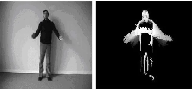
The main idea is creating a vector-image to be able to match it against stored representations of known movements. Therefore, we first segmented the action from the background image using background subtraction method. Then we extracted Motion history images (MHI) from segmented video sequences that allow representing the motion in multiple frames in a more powerful way. A sample video sequence consisting of ten frames is shown in Figure.3.1 (a) with MHI in Figure3.1 and 3.2, respectively.

Source: Schuldt C., Laptev I., Caputo B., 2004

Figure 3. 1 : Running Man

(24)

Figure 3. 2 : Mhi of running man

In order to evaluate the accuracy of our system, we divided our data into two as training and test sets, where we have 80 samples for training and 80 samples for testing, for each action. We used PCA and LDA as feature extraction methods, and SVM and KNN as classifiers and tested the accuracy of the system for different combinations using a feature extractor and a classifier.

3.1 BACKGROUND SUBTRACTION

One of the basic methods for motion detection in video sequences is background subtraction. In this method, corresponding pixels of two frames is compared, and their differences is taken and the pixels which their value more than a certain threshold are changes pixels (McIvor 2000). Moving objects are those whose pixel values have changed significantly.

Therefore, after comparing the corresponding pixels, all connected components (objects) that have fewer than P pixels, where P is the threshold value determined experimentally as 15 are removed from the images. Because it was assumed that these are the pixels that don’t belong to the motion.

(25)

Figure 3. 3 : Orginal frame

(26)

Figure 3. 5 : After removing noisy pixels

To make this technique suitable for real-time applications, it requires small memory space (one frame) and a small number of operations per pixel (integer subtraction), although this technique is not reliable for recognizing the moving object



 























otherwise

t

y

x

R

t

y

x

I

f

y

x

B

,

1 ,

,

0

1 ]

,

[

_(3.1)

I[x, y, t+1] is values of t+1 image frame. R[x, y, t] is values of t frames

Although the background is static, the motion region can be isolated from the background by first capturing the background image and then subtracting it from each subsequent frame. While subtracting each subsequent frames, we removed small sized objects after performing connected components labelling followed by a threshold based on area. Pixel groups that are not connected to a component more than 15 pixels are removed to segment the motion from video sequences in the best way. In the end of this step we had subsequent frames to constitute MHI.

(27)

3.2 WHAT IS MHI?

The image that obtained by squashing the image-time volume onto a single image is named as MHI. The intensity values in the MHI shows the time of the pixels which last motion happened or object presence. It represents motion the image is moving Ht, pixel intensity is a function of the temporal history of motion at that point. MHI‘s were calculated for 0-t time period for each motion, after motion was extracted from video frames. An advantage of MHI is that although it is a representation of the history of pixel-level changes, only one previous frame needs to be stored. (Bobick & James 2001)

For the results presented here, we use a simple replacement and decay operator:

          otherwise 1 y) D(x, if 1) 1) t y, (x, max(0, T

H

t t (3.2)

The result is a scalar-values image. More recently changed pixels are shown brighter. Examples for MHIs are presented in Figure 3.6, 3.7, 3.7 and, 3.9

(28)

Figure 3. 6 : Running man

Figure 3. 8 : Handclapping man

Figure 3. 9 : Mhi of handclapping man

(29)

3.3 WHAT ARE HU MOMENTS?

The use of moments as invariant binary shape representations was first proposed by Hu (1962). He classified handwritten characters successfully by using this technique.Hu moments show that recognition schemes based on these invari

position, size and orientation independent, and also flexible enough to learn almost any set of patterns. The concept of moments is used extensively in classical mechanics and statistical theory. In addition to this that, central moment

principal axes are also used.

In the pattern recognition field, centroid and size normalization have been exploited for “pre-processing.” Orientation normalization has also been attempted. The Hu moments presented here achieves o

absolute or relative orthogonal moment invariants. To characterize each pattern for recognition, the method uses “moment invariants” or invariant moments (moments referred to a pair of uniquely dete

Training examples of each movement running,

collected. Statistical descriptions of these images are computed by using moment features in a given set of MHIs for each movement combinat

Hu moments because of the fact that they are known to yield reasonable shape discrimination in a translation

The two-dimensional moment,

function, , (image intensity )is defined as

pq m

 

      

3.3 WHAT ARE HU MOMENTS?

The use of moments as invariant binary shape representations was first proposed by Hu (1962). He classified handwritten characters successfully by using this technique.Hu moments show that recognition schemes based on these invari

position, size and orientation independent, and also flexible enough to learn almost any set of patterns. The concept of moments is used extensively in classical mechanics and statistical theory. In addition to this that, central moments, size normalization, and principal axes are also used.

In the pattern recognition field, centroid and size normalization have been exploited for processing.” Orientation normalization has also been attempted. The Hu moments presented here achieves orientation independence without ambiguity by using either absolute or relative orthogonal moment invariants. To characterize each pattern for recognition, the method uses “moment invariants” or invariant moments (moments referred to a pair of uniquely determined principal axes)

Training examples of each movement running, handclapping,

collected. Statistical descriptions of these images are computed by using moment features in a given set of MHIs for each movement combination. Our cu

moments because of the fact that they are known to yield reasonable shape discrimination in a translation- and scale-invariant manner.

dimensional moment,m_pq of order p +q of a density distribution

, (image intensity )is defined as

y x q p_y _f _x _y _d _d x ( , )



 

The use of moments as invariant binary shape representations was first proposed by Hu (1962). He classified handwritten characters successfully by using this technique.Hu moments show that recognition schemes based on these invariants could be truly position, size and orientation independent, and also flexible enough to learn almost any set of patterns. The concept of moments is used extensively in classical mechanics and s, size normalization, and

In the pattern recognition field, centroid and size normalization have been exploited for processing.” Orientation normalization has also been attempted. The Hu moments rientation independence without ambiguity by using either absolute or relative orthogonal moment invariants. To characterize each pattern for recognition, the method uses “moment invariants” or invariant moments (moments

handclapping, boxing, jogging is collected. Statistical descriptions of these images are computed by using moment-based ion. Our current choice is 7 moments because of the fact that they are known to yield reasonable shape

+q of a density distribution

(30)

The central moments  are defined as_pq 

 

, ( ) ( )                        



x x y y p x y d x x d y y q p pq  (3.4) Where 00 10 m m x 00 01 m m y  (3.5)

It is well-known that under the translation of coordinates, the central moments do not change, and are therefore invariants under translation. It is quite easy to express the central moments  in terms of the ordinary moments _pq mpq for the first four orders, we

have 



₀₀moo  (3.6) 0 10



(3.7) 0 01



(3.8) 2 2 20    



m o (3.9)  

(31)

2 02 02   m y



(3.11) 3 20 3 30 3 2     m_o m  x



(3.12)        m m y m x x y 2 11 20 21 21 2 2



(3.13) 2 11 02 12 12 2 2        m m  m y x y



(3.14) 3 02 03 03 3 2     m m y y



(3.15)

To achieve invariance with respect to orientation and, scale, we first normalize for scale defining :_pq _    00 pq pq  (3.16)

Where  (pq)/21 and p q2 the first seven-orientation invariant Hu moments are defined as:

₁ ₂₀ ₀₂ (3.17) 2 11 2 02 20 2 (  ) 4     (3.18)

(32)

2 03 21 2 12 30 3 ( 3 ) (3  )      (3.19) 2 03 21 2 12 30 4 (  ) (  )      (3.20)











2



03 21 2 12 30 03 21 21 21 2 03 21 2 12 03 12 30 2 12 30 5 ) ( 3 ) )( 3 ( ) ( 3 ) ( ) ( ) 3 (                              (3.21) ) )( ( 4 ) ) ( ) (( ) ( 11 30 12 21 03 2 03 21 2 12 30 02 20 6                     (3.22)







2



03 21 2 12 30 03 21 12 30 2 03 21 2 12 30 12 30 03 21 7 ) ( ) ( 3 ) )( 3 ( ) ( 3 ) ( ) )( 3 (                              (3.23)

These moments can be used for pattern identification independent of position, size, and orientation.

(33)

3.4 FEATURE EXTRACTION

Feature extraction involves simplifying the amount of resources required to describe a large set of data accurately. When performing analysis of complex data one of the major problems stems from the number of variables involved. Analysis with a large number of variables generally requires a large amount of memory and computation power or a classification algorithm which over fits the training sample and generalizes poorly to new samples. Feature extraction is a general term for methods of constructing combinations of the variables to get around these problems while still describing the data with sufficient accuracy.

3.4.1 Principle Component Analysis (PCA)

One of the image classification techniques used for the face recognition is Principle Component Analysis (PCA). The most of descriptive features of an image are principal components. In this method, a new set of variables, that is called principal components, are generated. Each if this principal component is a linear combination of the original variables. All the principal components are orthogonal to each other, so there is no redundant information. The principal components as a whole form an orthogonal basis for the space of the data here are an infinite number of ways to construct an orthogonal basis for several columns of data. The main advantage of PCA is compressing data by reducing the number of dimensions without much losing of data information. The second one is identification of groups of inter-related variables, to see how they are related to each other. On the other hand, the main disadvantage of PCA is that it is only able to searching for linear relationships in the data. When the data is clustered, it might be more useful to apply PCA. Furthermore, the other main disadvantage of PCA is to have high computational complexity for large data sets (Lie-Wei et al. 2005).

(34)

The first principal component is a single axis in space. Each observation on that axis results values form a new variables. And the variance of this variable is the maximum among all possible choices of the first axis.

The second principal component is another axis which is perpendicular to the first one. Observations on this axes generates another new variable. The variance of this variable gives the maximum among all possible choices of this axis.

The full set of principal components is as large as the original set of variables. But it is common place for the sum of the variances of the first few principal components to exceed 90% of the total variance of the original data. By examining plots of these few new variables, researchers often develop a deeper understanding of the driving forces that generated the original data.

Training procedure in any classification system is significant and can be beneficial. Using various algorithms training can be performed. Algorithm used in current image classifier system for training is principal component analysis, whose major emphasis is to locate and depict the principal features of the given sample image The Eigenvectors is a key capability used in PCA analysis algorithm. Eigenvectors are defined to be a related set of spatial characteristics that computer uses to recognize a specific motion type. PCA technique uses training and testing sets of images. Eigenvectors of the covariance matrix is computed from the training set of images. These eigenvectors represent the principal components of the training images. These eigenvectors are often ortho-normal to each other. In the context of clouds classification, these eigenvectors would form the motion space. They can be thought of as a set of features that together characterize the variation between motion images.

The description of PCA is below. The aim is to reduce data set X of dimension M to data set Y of dimension L. Put it differently, our goal is to achieve the values of matrix Y, which in other words Karhunen-Loeve transform (KLT) of matrix X.

(35)

) (X

KLT

Y  (3.24)

We have comprising data set observations of M variables and we want to reduce each observations to describe with L variables L<M. The data form isx ...₁ x_N. x_N

Represent a single grouped observation of the M variables. x ...₁ x_N Column vectors is placed to the matrix X of dimension M x N. After these operations, we calculate the empirical mean along dimension m=1...M and store mean values into mean vector u of dimensions M × 1.

 

_

 

  N n n m X N m 1 , 1  (3.25)

We subtract the mean vector  each column of the data matrix X and store data in the

M x N matrix B



  X

B (3.26)

Next step is to find covariance matrix from the outer product of matrix B with itself.





 

_. * 1 _B_._B* N B B E B B E C     (3.27)

E is the expected value operator,  is the outer product operator, and * is the conjugate transpose operator. After calculated covariance matrix, we find the eigenvectors and eigenvalues of the covariance matrix.

(36)

D CV V1 

(3.28)

V is the matrix of eigenvectors which diagonalizes the covariance matrix C.D is the diagonal matrix of eigenvectors of C. Matrix D‘s form is M x M diagonal matrix, where

 

p q m

D ,  For p=q=m (3.29)

is the mth eigenvalues of the covariance matrix C, and

 

p,q 0

D For p<>q (3.30)

Matrix V contains M column vectors, that have M length, which represent the M eigenvectors of the covariance matrix C. Eigenvectors and eigenvalues might be considered paired, the mth eigenvalue corresponds to the mth eigenvector then we sort the columns of the eigenvalue matrix D in order of decreasing eigenvalue, because eigenvalue represent distribution of the source data's energy among each of the eigenvectors. The cumulative energy g is calculated.

 

_

 

  m q q p D m g 1 , For p=q and m=1....M (3.31)

We use g vector to find value for L. We want to choose threshold such as %90 etc.



m L



%90

(37)

After these operations we normalize the data using empirical standard deviation vector s the from square root of each element along the main diagonal of the covariance matrix C

 

 

sm C

 

p q

s  , For p=q=m=1...M (3.33)

Z= (divide element by element) (3.34)

The last step is to project the data onto new feature space.

 

X KLT Z

W

Y  *.  _(3.35)

We used another dimension reduction algorithms called LDA using Hu moments features.

h s

B

(38)

3.4.2 Linear Discriminant Analysis (LDA)

Linear Discriminant Analysis (LDA) is the way for extracting features and dimension reduction of data for classification. LDA which maximizes the ratio of between-class variance to within-class variance in any particular data set finds the linear combination of features for separating two or more classes. LDA tries to divide region between classes. LDA wants to know the distribution of the feature data. The main advantage of LDA is that reduces the dimension of a data set to reveal its essential characteristics and also computing cost is very low compared with PCA and in addition to this, LDA shows powerful performance in the low dimension. However, LDA lose some discriminative information in the high dimensional space and furthermore, each class is thought to has a normal distributions with a common covariance matrix. (Balakrishnama & Ganapathiraju 1998)

The approach of LDA is about involving maximizing the ratio of overall variance to within class variance. Below Figure 3.5 shows good class separation

Figure 3. 10 : Class separation

This approach makes the data sets transform to use one optimizing criterion; hence all data points irrespective of their class identity are transformed using this transform. In this type of LDA, each class is considered as a separate class against all other classes.

(39)

The sample sets below are analyzed using LDA with the mathematical operations. This approach was applied to a two-class problem for easily understanding.

Set1 is data set and set 2 is the test sets, they are be classified in the original space. The data sets are represented as a matrix form that consist of features

                                          2 22 21 1 21 11 2 22 12 1 21 11 .. .. .. .. .. .. 2 .. .. .. .. .. .. set1 m m m m b b b b b b set a a a a a a (3.36)

Both the mean of each data and mean of entire data set must be calculated. V1 and V2 are mean of data set 1 and data set 2. V3 is also mean of the whole data.P1 and P2 are probabilities of the classes.

õ

p

õ

p

õ

3 ₁ 1 ₂ 2 (3.37)

In LDA, within-class and between-class scatter are calculated for the class separability. Within-class scatter is measured by covariance of each of the classes

) (

_cov

_j

j

w p

s





 (3.38)

Therefore, for the two-class problem,

5 . 0 5 . 0 xCOV COV

s

   (3.39)

(40)

One of the properties of the covariance matrices are symmetric.COV1 and COV2 represent the covariance of data set 1 and data set 2. Covariance matrix is calculated using the following equation.

T j j j j j (

x

)(

x

)

cov

 







(3.40) The following equation calculates the between-class scatter.

T j j j b

S

( ) ( ) 3 3



   



(3.41)

The ratio of between-class scatter to the within-class scatter is the optimizing criterion of LDA. This criterion must be maximized to reach solution. This solution defines the axes of the transformed space. In addition to this, equations 3.42 and 3.41 are used to compute the optimizing criterion for the class-dependent transform. The optimizing factor is measured for class dependent type using below equations

S

inv

criterion

j (cov j ) b (3.42)

For the class independent transform, the optimizing criterion is computed as

 

s

_w

xs

_b

inv

criterion



(3.43) An eigen vector that is a subspace of the vector space represents a 1-D invariant subspace and also this eigen vector is linearly independent. Linear dependency is represented by zero eigen value. Non-zero eigen values are considered and one of the

(41)

zero eigen values is neglected. The eigen vector matrix of the different criteria defined in Equations 3.42 and 3.43

We have L-1 non-zero eigen values for L-class problem. We transform the data sets using the single LDA transform or the class specific transforms whichever the case may be. The transforming the entire data set to one axis provides definite boundaries to classify the data. The decision region in the transformed space is a solid line separating the transformed data sets thus for the class dependent LDA,

j set x j transform j set d transforme _{_} _{_} _ _{_} t _{_} _(3.44)

For the class independent LDA,

T T _x _data _set spec transform set d transforme _  _ _ (3.45)

The Euclidean distance of the test vectors from each class mean is used to classify and to transform to the test vectors. Both the original data sets and transformed data set are showed. Transformation provides a boundary for classification. In this example the classes were properly defined but in other cases, there might be overlap between classes. In some case, defined decision region is very difficult and in such cases importance of the transformation is considered. Transformation along largest eigen vector axis is the best transformation.

Euclidean distance or RMS distance is used to classify data points after LDA transforms. Equation 3.34 shows how Euclidean distance is computed. _ntrans is the mean of the transformed data set, is n the class index and x is the test vector. N Euclidean distances are obtained for each test point for n classes.

(42)

ntrans T spec n transform n dist_  ( _ _ )   (3.46)

The smallest Euclidean distance among the distances classifies the test vector as belonging to class.

All the things we made to now are for classification to create database to compare new motion. We used two algorithms to recognize human motion. One of these is Support Vector Machines (SVM), another is knn classifier.

(43)

3.5 CLASSIFICATION

In the field of Machine Learning, the goal of classification is to group items that have similar feature values, into groups. A linear classifier achieves this by making a classification decision based on the value of the linear combination of the features.

In our thesis, we used K Nearest Neighbours and Support Vector Machines classifier for recognition and compared these techniques

3.5.1 K Nearest Neighbours

The k-nearest neighbours classifier is both the simplest of all machine learning algorithms and the simplest to implement. An object is classified by a closeness of its neighbours, with the object being assigned the class most common amongst its k nearest neighbours. K is a positive integer. If k is chosen one, then the object is belong to assigned the class of its nearest neighbours. It is helpful to choose k to be an odd number as this avoids difficulties with tied votes (Venkatesh & Ramakrishnan 2004)

The main advantage of KNN classifier is the simplest to implement and also K-nearest can predict both qualitative attributes that is the most frequent value among the k nearest neighbours and quantitative attributes that is the mean among the k nearest neighbours. In addition to this, it doesn’t require creating a predictive model for each attribute with missing data and takes in consideration the correlation structure of the data. Furthermore it has robust performance.

On the other hand, KNN can have poor run-time performance if the training set is large, KNN is very sensitive to irrelevant or redundant features and also slow testing and scale (metric) dependent.

(44)

3.5.2 Support Vector Machines

Support vector machines (SVMs) being a sentence in connection standing supervised learning methods, those for classification and regression. They belong to a family of the generalized linear classifier and can be supposed as a special case of the Tikhonov regularization. A special characteristic from SVMs is that they lower the empirical classification error at the same time and maximize the geometrical side edge; therefore they are alias maximum margin classifiers. The main advantage of SVMs is the possibility to provide greater generalization performance using nonlinear classifiers in high dimensional spaces over a small training set. The input dimensionality of the problem is not related to the error of the SVMs; however the margin separates the data. This indicates SVM’s good performance even with a large number of inputs. However, SVM has limitations that are speed, size both in training and test data. SVMs is the high algorithmic complexity and extensive memory requirements (Christopher & Burges 1998)

Support vector machines diagram entrance vectors to a higher measure area, in which a maximum separating hyper plane is designed. Two parallel hyper levels are designed on each side of the hyper level, which separates the data. The separating hyper level is the hyper level, which maximizes the distance between the two parallel hyper levels. An acceptance is formed that, which more largely the side edge or the distance between these parallel hyper levels, which is better the generalisation error of the classifier. A comparison of the SVM to other classifiers through van der Walt and Barnard pool of broadcasting corporations are accomplished frequently a machine-learning process is used by us to classify data. Each data point belonging to only one of two categories is showed by a P-dimensional vector (a list of the p numbers). We would like to see if we can separate them with a "p minus 1" measure hyper plane. This is a typical form of the linear classifiers. There are many linear classifiers, which could fulfil this characteristic. However we additionally interested, on to find out, if we can obtain maximum separation (margin) between the two categories. By this we mean that we select the hyper plane, so that the distance from the hyper plane to the next data point is

(45)

maximized. That is called that the next distance between one point in a separate hyper plane and one point in the other separate hyper plane is maximized.

Data points of the form is regarded



(

_x

₁

,

_c

₁

),

(

_x

₂

,

_c

₂

),...,

(

_xn

,

_cn

)



(3.47) Where ci is either 1 or -1, a constant showing the class where the point Xi belongs Xi is a p-dimensional real vector which normalize [0, 1] or [-1, 1] values. To save against variables (attributes) with larger variance may control classification. We can called this as training data, that indicate the correct classification by means of the dividing (or separating) hyper plane, which takes the form

source: http://en.wikipedia.org/wiki/Support_vector_machine [cited 28 June 2007]

Figure 3. 11 : Maximum-margin hyper planes for a SVM

Maximum-margin hyper planes for a SVM trained with samples from two classes. Samples along the hyper planes are called the support vectors.

(46)

0 





x

b

w

(3.48)

The vector w represents the perpendicular to the separating hyper plane. Adding the parameter b is to increase the margin. In its absence, it makes the hyper plane pass through the origin, restricting the solution.

When we look at in the maximum margin, we are interested in the support vectors. Parallel hyper planes are closest to these support vectors in either class. The below equations show these parallel hyper planes

. 1 , 1        b x w b x w (3.49)

If we separate linearly the training data, we can select these hyper planes. There are no points between them and then try to maximize their distance. By using geometry, we minimize |w|, and find the distance between the hyper planes is 2/|w|. We need to ensure that for all I either

, 1 1      

b

x

w

x

w

i i or (3.50)

This can be rewritten as:

n i b

x

w

c

i(  i )1 , 1  (3.51)

Primal form, the problem now is to minimize |w| subject to the constraint (1). Minimize (1 2) w2, subject to

(47)

n i

b

x

w

c

i(  i )1, 1  (3.52)

The factor of ½ is used for mathematical convenience

Dual Form, writing the classification rule in its dual form reveals that classification is only a function of the support vectors, i.e., the training data that lie on the margin. The dual of the SVM can be shown to be

x

c

a

J T j i j j i i n i i



 1 , max Subject to

_a

_i0 (3.53)

Where the a terms constitute a dual representation for the weight vector in terms of the training set:

x

c

a

(48)

4. TESTING FEATURE EXTRACTION AND

CLASSIFICATION

Methodologies have been implemented on a database consisting of 80 video sequences of four different motions, i.e. running, jogging, boxing and handclapping (Schuldt, Laptev and Caputo, 2004). Common characteristic of all these videos is that the background is static and there is no object moving, except for human motion in all videos. All videos were taken with a static camera at 25fps frame rate and stored using AVI file format in RGB without compression each of which are approximately four seconds on average duration with a spatial resolution of 160x120 pixels leading to an average size of 1.5 megabytes.

In these videos, each different motion has been performed by four different people. We separated the dataset into two groups as training and testing sets to perform the recognition tests. Training set consists of randomly selected 80 video sequences, 20 for each distinct motion. It has been used to construct the feature space and train the particular classifiers as mentioned in Sections 3.4 and 3.5, respectively. The remaining 80 test samples have been used for testing using the methodology explained in detail in Section 3

4.1 MHI

The intensity values in the MHI are indicative of the time at which that pixel last witnessed motion or object presence. There are a few problems to create MHI of videos. The big problem is the repeating motion in video. During the training phase, we

measure the minimum and maximum duration that a movement may take, tminand tmax.

If the test motions are performed at varying speeds, we need to choose the right value for t for the computation of the MHI.

(49)

To choose right t is very important in handclapping videos since the human moving can repeat one more handclapping in one video. Therefore, we took first motion from the beginning frame to the end frame of first handclapping motion accordingly. Similar problems in jogging and running videos were handled in the same way. In such videos some people can run or jog in angle of camera between 0-t periods, where the camera can capture the returning motion of some people in the same period, too. Similarly, we only took first complete cycle of the action to avoid such problems. Although capturing first motion of boxing is very hard, we took just 4 frames of each boxing videos and created MHI’s using these frame periods. Figures 4.1, 4.2, 4.3 and 4.4 show some example MHIs constructed for boxing, hand clapping, jogging and running sequences, respectively.

(50)

Figure 4. 2 : Mhi of handclapping man

(51)

Once the MHI’s are constructed, they are used to compute seven Hu moments. These moments used to characterize these motions quantitatively. Besides, since Hu moments are invariant to translation, rotation and scale, we are not required to apply pre-processing such as resizing or moving the motion to centre of image frame. As mentioned in Section 3, Hu moments of each motion have been calculated and these values have been stored to create the training database, where they have been used as input for the feature extraction step using PCA and LDA. In our training database, first 20 samples correspond to boxing, samples between 21 and 40 correspond to handclapping, 41 and 60 represent to jogging and the rest 20 correspond to running actions.

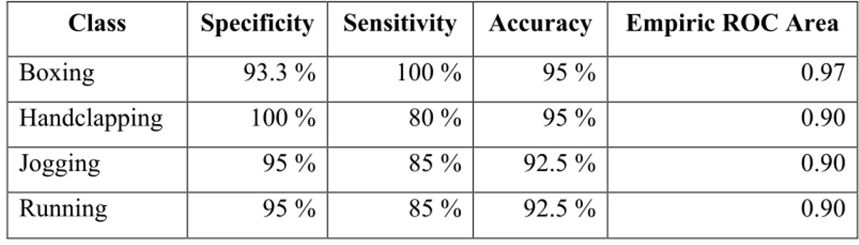
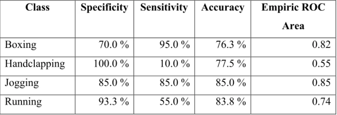
The final stage for human motion recognition is the classification step, where every test sample is classified using the parameters learned from the training data and the accuracy of the system is evaluated. Before applying any feature extraction step, first we performed an independent test to compare the classification accuracies of two classifiers: KNN and SVM, which are discussed in Sections 3.5.1 and 3.5.2. The independent test results for each motion have been presented in Tables 4.1 and 4.2.

(52)

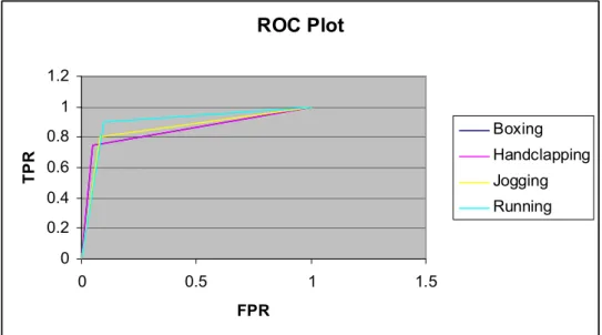
Table 4. 1 : The result of KNN classifier for each motion classes Class Specificity Sensitivity Accuracy Empiric ROC Area

Boxing 93.3 % 100 % 95 % 0.97

Handclapping 100 % 80 % 95 % 0.90

Jogging 95 % 85 % 92.5 % 0.90

Running 95 % 85 % 92.5 % 0.90

As can be seen from the results reported in Table 4.1 and Figure 4.5, the proposed approach was able to classify all four types of human activities with a remarkable overall accuracy of 93.8 percent using the KNN classifier. Classifying all boxing sequences correctly, the system was most sensitive on detecting samples of this action with 100 percent perfect accuracy. However, the specificity of this type of action is the lowest as expected. On average, both the overall specificity and sensitivity; therefore the overall classification accuracy of the system as indicated by the ROC area under the curve was significantly high, meaning the system was quite accurate identifying human actions of different types from video sequences.

Figure 4. 5 : ROC Curve for each classes with KNN classifier

ROC Plot 0 0.2 0.4 0.6 0.8 1 1.2 0 0.5 1 1.5 TPR F P R Boxing Handclapping Jogging Running

Human motion analysis and action recognition

T.C.

BAHÇEŞEHİR ÜNİVERSİTESİ