YAŞAR UNIVERSITY
GRADUATE SCHOOL OF NATURAL AND APPLIED SCIENCES MASTER THESIS
A COMPARISON OF THE PERFORMANCE OF
ENSEMBLE CLASSIFICATION METHODS IN
TELECOM CUSTOMER CHURN ANALYSIS
Gökçe KALABALIK
Thesis Advisor: Prof. Dr. Mehmet Cudi OKUR
Department of Computer Engineering
Presentation Date: 03.03.2016
Bornova-İZMİR 2016
iii ABSTRACT
A COMPARISON OF THE PERFORMANCE OF ENSEMBLE CLASSIFICATION METHODS IN TELECOM CUSTOMER CHURN
ANALYSIS KALABALIK, Gökçe MSc in Computer Engineering Supervisor: Prof. Dr. Mehmet Cudi OKUR
March 2016, xx pages
Data mining is used to analyze mass databases in order to discover hidden information. Churn analysis based on classification is one of the most common applications of data mining. It is used to predict the behavior of customers who are most likely to change the provided telecom service. In this way, specific campaigns can be created for them. Customer churn is one of the most significant problems that affect business nowadays. The main purpose of churn prediction is to classify the customers into two types. These two types are customers who leave the company and customers who continue doing their business with the company. In order to identify future churners, predictive models based on past data can be developed. However, it has become more difficult to assess the proper classification methods for churn prediction applications since the number of classification models have also increased. In the area of telecom churn prediction, conventional statistical prediction methods are used mostly. This thesis examines combining multiple machine learning algorithms using ensemble methods to increase the accuracy measures of the existing prediction methods. The major aim is to evaluate classification results in telecom customer churn management using bagging, boosting, and random forest ensemble classification methods. Weka software tool has been used to evaluate the performance of common bagging, boosting, and random forest techniques. The results indicate moderate improvements in classification accuracies and other measures. Based on the results, it can be said that ensemble methods with a good base learner are efficient in churn classification. This thesis comprises of eight sections which include these subjects, their applications, and the results.
Keywords: Data Mining, Churn Analysis, Telecom Churn, Classification, Ensemble Methods, Bagging, Boosting, Random Forest
iv ÖZET
TELEKOMÜNİKASYON SEKTÖRÜ MÜŞTERİ AYRILMA ANALİZİNDE BİRLEŞTİRMELİ SINIFLANDIRMA YÖNTEMLERİ
PERFORMANSLARININ KARŞILAŞTIRILMASI Gökçe KALABALIK
Yüksek Lisans Tezi, Bilgisayar Mühendisliği Bölümü Tez Danışmanı: Prof. Dr. Mehmet Cudi OKUR
Mart 2016, xx sayfa
Veri madenciliği, saklı bilgiyi ortaya çıkarmak için büyük veri kümelerini analiz etme sürecidir. Sınıflandırmaya dayanarak yapılan müşteri ayrılma analizi veri madenciliğinin en yaygın uygulama alanlarından biridir. Bu analiz, telekomünikasyon servis sağlayıcılarını değiştirme eğilimi gösteren müşterilerin tutumunu tahmin etmekte kullanılır. Böylelikle, bu müşteriler için özel kampanyalar oluşturulabilir. Günümüzde, ayrılacak müşteriler iş hayatını etkileyen en önemli problemlerden biridir. Müşteri ayrılma analizinin esas amacı müşterileri iki tipte sınıflandırmaktır. Bu iki tip müşteri; şirketten ayrılanlar ve şirketle işlerini yürütmeye devam edenlerdir. Gelecekte şirketten ayrılma eğilimi olan müşterileri saptamak için geçmiş verilere dayalı tahmin edici modeller geliştirilebilir. Bununla birlikte, sınıflandırma yöntemlerinin sayısı arttığından dolayı müşteri ayrılma analizi tahmini uygulamaları için uygun sınıflandırma yöntemlerini belirlemek daha da zor bir hal aldı. Telekomünikasyon sektöründe müşteri ayrılma analizi tahmininde, geleneksel istatistiksel tahmin yöntemleri çoğunlukla kullanılmaktadır. Bu tez, çoklu makine öğrenmesi algoritmalarının, birleştirmeli sınıflandırma yöntemlerini mevcut tahmin etme metotlarının ölçü doğruluğunu artırmak için kullanarak birleştirilmesini inceler. Başlıca amaç, bagging, boosting ve random forest birleştirmeli sınıflandırma yöntemlerini kullanarak telekomünikasyon sektöründe müşteri ayrılma yönetimi sınıflandırma sonuçlarının değerlendirmeye alınmasıdır. Yaygın bagging, boosting ve random forest tekniklerinin performansını değerlendirmek için Weka yazılım aracı kullanılmıştır. Sonuçlar sınıflandırma doğrulukları ve diğer ölçülerde makul iyileşmelere işaret etmektedir. Sonuçlara dayanarak, iyi bir sınıflandırma tabanı ile kullanılan birleştirmeli sınıflandırma yöntemlerinin müşteri ayrılma analizi tespitinde etkili olduğunu söylemek mümkündür. Bu tez; bu konuları, uygulamalarını ve sonuçlarını içeren sekiz bölümden oluşmaktadır.
v
Anahtar sözcükler: Veri Madenciliği, Müşteri Ayrılma Analizi, Telekomünikasyon Sektöründe Müşteri Ayrılma Analizi, Sınıflandırma, Birleştirmeli Sınıflandırma Yöntemleri, Bagging, Boosting, Random Forest
vi
ACKNOWLEDGEMENTS
I would like to thank to my supervisor Prof. Dr. Mehmet Cudi OKUR for his guidance and support throughout the research and writing phases of my thesis.
Furthermore, I would like to thank to the academic staff of Computer Engineering and Software Engineering Departments of Yaşar University, for their interest in my work and in my seminar presentation which gave me an opportunity to put my theoretical knowledge into practice.
Finally, I would like to thank to my parents for their constant support.
Gökçe KALABALIK İzmir, 2016
vii
TEXT OF OATH
I declare and honestly confirm that my study, titled “A Comparison of the Performance of Ensemble Classification Methods in Telecom Customer Churn Analysis” and presented as a Master’s Thesis, has been written without applying to any assistance inconsistent with scientific ethics and traditions, that all sources from which I have benefited are listed in the bibliography, and that I have benefited from these sources by means of making references.
viii TABLE OF CONTENTS Page ABSTRACT iii ÖZET iv ACKNOWLEDGEMENTS vi
TEXT OF OATH vii
TABLE OF CONTENTS viii
INDEX OF FIGURES xi
INDEX OF TABLES xiv
INDEX OF SYMBOLS AND ABBREVIATIONS xv
1 INTRODUCTION 1
2 LITERATURE REVIEW 3
3 CLASSIFICATION MODELS 7
Decision Trees 7
Rule Based Classifiers 11
Other Classification Methods 11
Neural Networks Based Classification 11
ix
Performance Evaluation Methods 14
Confusion Matrix Based Performance Measures 15
Receiver Operating Characteristic Curve 17
Error Rates 18 4 Ensemble Methods 19 Bagging 22 Boosting 23 Random Forest 25 5 IMPLEMENTATION 27 Dataset Description 27
Dataset Variables Selection 28
6 Experimental Results 30
Base Classifiers: Decision Stump and J48 Implementation 30
Decision Stump for Full Data Set 30
J48 Decision Tree for Full Dataset 32
Implementation Results of Bagging Ensemble Classification 34
6.2.1 Bagging-Decision Stump Base-Full Dataset 34
x
6.2.3 Reduced Dataset Bagging-J48 Decision Tree Base 37 Implementation Results of Boosting Ensemble Classification 38
Boosting-Decision Stump Base-Full Dataset 38
Boosting-J48 Decision Tree Base-Full Dataset 40
Reduced Dataset Boosting-J48 Decision Tree Base 41 Implementation Results of Random Forest Ensemble Classification 42 6.4.1 Random Forest Classification for Full Dataset 42 6.4.2 Random Forest Classification for Reduced Dataset 43 7 Evaluation of the Ensemble Classification Methods Based on Weighted
Performance Values 45
Accuracy Measures 45
7.1.1 Decision Stump Base Implementation Accuracy Results Comparisons 46 7.1.2 J48 Base Implementation Accuracy Results Comparisons 48 7.1.3 Reduced Dataset Implementation Accuracy Results Comparisons 50
Error Rate Comparisons 52
8 CONCLUSION AND FUTURE WORK 58
REFERENCES 59
xi
INDEX OF FIGURES
Figure 3.1 A simplified churn prediction decision tree (Almana et al., 2014) 8 Figure 3.2 Decision Tree Learning Algorithm (Almana et al., 2014) 9 Figure 3.3 An example of a decision stump on Irish flower dataset 10 Figure 3.4 A decision tree for the concept buys computer (Han and Kamber, 2006) 10 Figure 3.5 Real Neuron and Artificial Neuron Model (Larose, 2005) 12
Figure 3.6 Maximum Margin Hyperplane 14
Figure 3.7 Different Outcomes of a Two-Class Prediction 15
Figure 3.8 ROC Curve 17
Figure 4.1 General Idea of Ensemble Methods 19
Figure 4.2 An ensemble of linear classifiers (Oza, 2009) 21 Figure 4.3 An ensemble of linear classifiers (Oza, 2009) 23
Figure 4.4 AdaBoost Algorithm 24
Figure 4.5 Random Forest 26
Figure 5.1 Statistical report of churn dataset (Vis et al., 2009) 27 Figure 5.2 Final optimal subset of features (Kozielski et al., 2015) 29 Figure 6.1 Weka Output of Decision Stump Algorithm on the Full Dataset 31 Figure 6.2 ROC Curve of Decision Stump Algorithm on the Full Dataset 31 Figure 6.3 Weka Output of J48 Algorithm on the Full Dataset 32
xii
Figure 6.4 ROC Curve of J48 Algorithm on the Full Dataset 32 Figure 6.5 Weka Output of Bagging Decision Stump Base on the Full Dataset 34 Figure 6.6 ROC Curve of Bagging Decision Stump Base on the Full Dataset 35 Figure 6.7 Weka Output of Bagging J48 Base on the Full Dataset 36 Figure 6.8 ROC Curve of Bagging J48 Base on the Full Dataset 36 Figure 6.9 Weka Output of Bagging J48 Base on the Reduced Dataset 37 Figure 6.10 ROC Curve of Bagging J48 Base on the Reduced Dataset 37 Figure 6.11 Weka Output of Boosting Decision Stump Base on the Full Dataset 38 Figure 6.12 ROC Curve of Boosting Decision Stump Base on the Full Dataset 39 Figure 6.13 Weka Output of Boosting J48 Base on the Full Dataset 40 Figure 6.14 ROC Curve of Boosting J48 Base on the Full Dataset 40 Figure 6.15 Weka Output of Boosting J48 Base on the Reduced Dataset 41 Figure 6.16 ROC Curve of Boosting J48 Base on the Reduced Dataset 41 Figure 6.17 Weka Output of Random Forest on the Full Dataset 42 Figure 6.18 ROC Curve of Random Forest on the Full Dataset 43 Figure 6.19 Weka Output of Random Forest on the Reduced Dataset 43 Figure 6.20 ROC Curve of Random Forest on the Reduced Dataset 44 Figure 7.1 Accuracy Measures for Full Dataset Decision Sump Base Implementation
xiii
Figure 7.2 Accuracy Measures for Full Dataset J48 Base Implementation Results 49 Figure 7.3 Accuracy Measures for Reduced Dataset Implementation Results 51 Figure 7.4 Error Rates for Full Dataset Decision Stump Base Implementation Results
53 Figure 7.5 Error Rates for Full Dataset J48 Base Implementation Results 55 Figure 7.6 Error Rates for Reduced Dataset Implementation Results 57
xiv
INDEX OF TABLES
Table 7.1 Accuracy Results Comparisons for Decision Stump Base Implementation 46 Table 7.2 Accuracy Results Comparisons for J48 Base Implementation 48 Table 7.3 Accuracy Results Comparisons for Reduced Dataset 50 Table 7.4 Decision Stump Base Error Rate Results Comparisons 52
Table 7.5 J48 Base Error Rate Results Comparisons 54
xv
INDEX OF SYMBOLS AND ABBREVIATIONS Abbreviations
PCT Percentage
RF Random Forest
1
1 INTRODUCTION
Data mining explores large, high-dimensional, and multi-type data sets that have meaningful structure or patterns with the help of statistical and computational methodologies. The fundamental purpose of data mining is to support the discovery of patterns in data to transform information into knowledge. Another purpose is to support decision making process or to explain and justify it. Availability of qualified data on business activities, integration of data repositories into data warehouses, the exponential increase in data processing and storage capabilities, and decrease in cost have led to the rapid development of data mining applications. In today’s competitive business world, data mining applications have become so widely used due to the more intense competition at the global scale and the need of making accurate and timely decisions. Data mining focuses on finding interesting and meaningful patterns from large datasets. For this reason, there have also been numerous scientific, health and security related applications.
Nowadays, huge amounts of data are being collected and warehoused. The amount of available data has increased and it has provided the opportunity to automatically find and uncover valuable information and to transform it into valuable knowledge. As computers have become cheaper and more powerful, competitive pressure has been stronger. With the widespread use of low-cost massive data storage technologies and the Internet, large amounts of data have been available for analysis. The organizations that are capable of transforming data into information and knowledge can use them in order to make quicker and more effective decisions and thus to achieve a competitive advantage (Vercellis, 2009).
In today’s competitive business world, information and knowledge has become the absolute power for both launching and managing companies. In terms of strategic decision making, more reliable decision support systems and mechanisms with the aid of IT and automated business intelligence models are needed. In recent years, predicting customer churn with the purpose of retaining customers has received an increasing attention due to the competitive business environments.
For many companies, finding reasons of losing customers, measuring customer loyalty and regaining customer have become very important concepts (Gürsoy, 2010).
2
Companies usually create special marketing tools in order to avoid losing their customers since it is more challenging to obtain new ones.
The subject of this thesis is the evaluation of classification results in telecom churn analysis using bagging, boosting, and random forest ensemble methods. Throughout the thesis; the classification models, decision trees, rule based classifiers, and other classifiers are reviewed in order to identify common approaches within the context of data mining. Afterwards, bagging, boosting, and random forest ensemble methods are explained. All of the algorithms are implemented in Weka 3.7 software tool which is comprised of a collection of machine learning algorithms developed at the University of Waikato in New Zealand. In the implementation phase, initially the dataset is introduced. Telco churn dataset has 3332 customer records with 21 attributes. It is a complete dataset which has no missing values for each attribute throughout all the records. After introducing the features, Decision Stump and J48 algorithms under the trees section within Weka classifiers are implemented separately on the full dataset. After that, Bagging and AdaBoostM1 algorithms under the meta section and Random Forest algorithm under the trees section within Weka classifiers are implemented separately. For the algorithms Bagging and AdaBoostM1 each of DecisionStump and J48 algorithms are used as the base algorithms. Afterwards, the same algorithms are used with a reduced dataset which includes most effective attributes for classification tasks. According to feature selection models, the optimal reduced number of the attributes is decreased to 11. (Kozielski et al., 2015). After completing all the implementation phases within Weka, the results are evaluated using common performance evaluation methods. The evaluation criteria include the following measures and statistics: The percentage of correctly classified instances, the percentage of incorrectly classified instances, true positive rate, and precision, F Measure, ROC Area and Kappa Statistic. The computed values are compared for each base algorithm, bagging, boosting, and random forest results. In terms of error rates, MAE (Mean Absolute Error), RMSE (Root Mean Squared Error), RAE (Relative Absolute Error) and RRSE (Root Relative Squared Error) values are compared for each base algorithm, bagging, boosting, and random forest results. Based on these metrics, comparison results and evaluations of the methods are presented.
3
2 LITERATURE REVIEW
The fundamental aim of customer churn prediction is identifying customers with a high tendency to leave a company. Customer churn is a common concern of most companies in business environments. Churn occurs when a customer leaves a company. It is a significant issue for most businesses since keeping an existing customer is cheaper than finding a new one. The company can focus on likely churners and try to keep them in case churn can be predicted. From the customer churn perspective, customers can be classified into two types churners and non-churners. Customers who leave the company are called as churners, whereas customers who continue their business with the company are called as non-churners. Improvement of churn prediction can increase profit of the company. The telecommunication industry is dynamic with a large base of customers. Among all industries which suffer from this issue, telecommunications industry can be considered in the top of the list with approximate annual churn rate of 30% (Jahromi, 2009).
The telecommunication industry is dynamic with a large base of customers. Churn prediction and management have become a significant issue especially for the mobile operators. As Gürsoy (2010) indicates the telecommunications sector acquires huge amount of data because of the rapidly changing technologies, the increase in the number of subscribers and many value added services. Due to the uncontrolled and rapid spreading of this field, losses have also increased. Therefore, it has become vital for the operators to acquire the amount invested and to gain at least a minimum profit within a very short period of time (Umayaparvathi et al., 2012). With the help of identification methods, customers who have a tendency to leave a telecom service provider preventive measures can be taken beforehand.
Mobile operators aim to keep their customers and satisfy their needs. To achieve this, they need to predict the customers who have a tendency to churn and then make use of the limited resources to retain those customers. In the telecommunication industry, classification and other data mining methods are used to reveal their profitable and stable customers. Classification methods mainly focus on predicting the customers who have a tendency to leave a certain company based on the user characteristics, user behaviors and quality of services. Developing effective strategies to win more customers and to retain the existing ones contribute to the
4
survival and good profitability of telecom companies. With the help of these strategies, a telecom company can grow and manage a large customer base to increase profits via telecommunication services like voice data transmission and broadband in a mass scale. However, in order to develop such kind of strategies, the reasons should be known why an existing customer chooses to discontinue his/her telecommunication company. It is very critical to identify churning timely for a company to keep pace with competitive and up-to-date telecommunication industry, in today’s dynamic business world, with rapid advances of related technologies, products, and services.
Companies in telecommunication industry have detailed call records within their databases. In their study Rygielski, Wang, Yen et al. (2002) presented that these companies can segment their customers by using call records for developing price and promotion strategies. By making use of data mining techniques, the customers who have a tendency not to make any payments can be detected beforehand. In this way, financial loss of telecom companies can also be reduced. Deviation determination method is one of the methods that is used for these types of analysis. Customers are divided into clusters according to their usage patterns. Customers with inconsistent features are detected and preventive measures are initiated for them.
Within their study; Ren, Zeng, and Wu (2009) presented a clustering method based on genetic algorithm for telecommunication customer subdivision. Initially, the features of telecommunication customers like calling and consuming behavior are extracted. Afterwards, the similarities between the multidimensional feature vectors of telecommunication customers are computed and mapped as the distance between samples on a two-dimensional plane. Eventually, the distances are adjusted to approximate the similarities gradually by genetic algorithm.
Analysis results from a big Taiwan telecom provider pointed out that the proposed approach has pretty good prediction accuracy by using customer demography, billing information, call detail records, and service changed log to build churn prediction mode by making use of Artificial Neural Networks (Chang, 2009).
In their study, Abbasimehr et al. (2014) indicate that as the results show the application of ensemble learning has brought a significant improvement for individual base learners in terms of three performance indicators i.e., AUC,
5
sensitivity, and specificity. Boosting gave them best results among all other methods. These results indicate that ensemble methods can be a best candidate for churn prediction tasks (Abbasimehr et al., 2014).
As Almana et al. (2014) pointed out within their study, decision tree based techniques, neural network based techniques and regression techniques are generally applied in customer churn.
Hung et al. (2006) indicated that both decision tree and neural network techniques can deliver accurate churn prediction models by using customer demographics, billing information, contract/service status, call detail records, and service change log.
Ensemble learning algorithms have received an increasing attention over last several years. Since these algorithms generate multiple base models using traditional machine learning algorithms and combine them into an ensemble model, their performance is usually better than single models. Amongst the ensemble learning algorithms, bagging and boosting are two of the most popular algorithms due to their good empirical results and theoretical support. An obvious approach to making decisions more reliable is to combine the output of several different models and several machine learning techniques. By learning an ensemble of models and using them in combination; they can often increase predictive performance over a single model. These are general techniques that are able to be applied to most classification tasks and numeric prediction problems (Witten et al., 2011).
Throughout this thesis, an ensemble method which originates from statistical machine learning called bagging (Breiman, 1996) is used. It consists of sequentially computing a base classifier from resampled versions of the training sample in order to obtain a committee of classifiers (Lemmens and Croux, 2006). The final classifier is then obtained by taking the average over all committee members. Applying bagging algorithm on a database is simple and easy even it requires a bit more computation time; it does not need any extra information when compared to the one training sample needs. As Lemmens and Croux (2006) reflect, there is a growing literature showing that committees usually perform better than the base classifiers. Breiman (1996) suggests classification tree as the base classifier. As Lemmens and Croux
6
(2006) point out more sophisticated versions of bagging with the use of weighted sampling schemes exist under the name of boosting.
The boosting ensemble method which is used throughout this thesis is Real Adaboost (Freund and Schapire, 1996). The main principle of boosting comprises of sequentially applying the base learner to adaptively reweighted versions of the initial dataset. It has been proposed that misclassified observations are assigned an increased weight in the next iteration and the weights given to previously correctly classified observations are reduced consequently (Lemmens and Croux, 2006). The main idea is based on forcing the classifier to focus on the instances which are difficult to classify. As Lemmens and Croux (2006) point out, boosting procedure requires software that allows assigning weights to the observations of the training sample when computing the base classifier. Lemmens and Croux (2006) also reflect that a key difference between bagging and boosting is the initial classification rule which is preferably a weak learner, for instance; a classifier that has a slightly lower error rate than random guessing. Lemmens and Croux (2006) indicate that using decision stumps for example binary trees with only two terminal nodes for Real Adaboost is suggested since such a weak base classifier would have a low variance but a high bias. As Lemmens and Croux (2006) point out after iterations of the boosting algorithm, the bias should be reduced, while the variance would remain moderate. In principle, boosting should therefore outperform bagging since it not only reduces the variance, but also the bias (Lemmens and Croux, 2006).
Random Forest is another ensemble method which is used throughout this thesis. Although it is under the trees section within Weka classifiers, it stands for a class of ensemble methods that is particularly designed for decision tree classifiers. Random Forest algorithm combines predictions made by plenty of decision trees. A popular algorithm for learning random forests builds a randomized decision tree in each iteration of the bagging algorithm, and often produces excellent predictors (Witten et al., 2011).
7
3 CLASSIFICATION MODELS
Decision Trees
Decision Tree is as a tree-shaped structure that depicts sets of decisions and produces rules for the classification of a dataset. It can also be described as a structure that is used to divide a large collection of records into sequentially smaller sets of records by applying a sequence of simple decision rules. Decision trees are based on divide-and-conquer concept. A decision tree consists of three types of nodes:
Root Node
Internal Node
Leaf or Terminal Node
As Clemente et al. (2010) state the fundamental logic behind Decision Tree is producing a classification of observations into groups and then obtaining a score for each group. CART (Classification and Regression Trees) algorithm is the most widely used tree algorithm amongst the statistical algorithms. CART analysis is based on predicting or classifying cases according to a response variable.
In terms of customer churn prediction, decision trees are the most common methods amongst the classification models. In order to evaluate a dataset using decision trees, classification is done by altering the tree until a leaf node is reached. When classifying customer records, class labels of churner or non-churner are assigned to the leaf node. Fig 3.1 illustrates a simplified decision tree for customer churn prediction in telecom sector.
8
Figure 3.1 A simplified churn prediction decision tree (Almana et al., 2014)
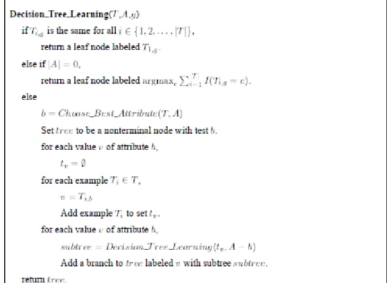
Decision trees has a top-down structure. A decision tree learning algorithm (ID3) is illustrated in Figure 3.2. If all the examples belong to the same class, the algorithm just returns a leaf node of that class. If there are no attributes left with which to produce a nonterminal node, then the algorithm has to return a leaf node. It returns a leaf node of the class which is most frequently seen in the training set. If none of them is true, then the algorithm finds the one attribute value test that comes closest to splitting the whole training set into parts such that each part only comprises of examples of one class. When such an attribute is chosen, the training set is split based on that attribute. It means that for each value of the attribute, a training set is produced such that all the examples in the set have value for the selected attribute. The learning algorithm is called recursively for each of the training sets.
9
Figure 3.2 Decision Tree Learning Algorithm (Almana et al., 2014)
Decision Stump and J48 are two of the widely used decision tree algorithms that are also used throughout this thesis. Decision Stump and J48 algorithms are under the trees section of Weka classifiers. A decision stump class comprises of a one-level decision tree with one root node that is instantly connected to the terminal nodes. A decision stump makes a prediction based on single criteria. In Figure 3.3, it can be observed that decision stump algorithm discriminates between two of three classes of Irish flower dataset. The value of petal width is measured in centimeters. Viola-Jones face detection algorithm employs AdaBoost with decision stumps as weak learners (Viola and Jones, 2004).
10
Figure 3.3 An example of a decision stump on Irish flower dataset
J48 is a class for generating a pruned or unpruned C4.5 decision tree. J48 is Weka’s implementation of C4.5 decision tree learner. J48 actually implements a later and slightly improved version called C4.5 revised version 8, which was the last public version of this family of algorithms before the commercial implementation C5.0 was released (Witten et al., 2011). ID3, C4.5, and CART adopt a greedy approach in which decision trees are constructed in a top-down recursive divide-and-conquer manner, in addition to this most algorithms for decision tree induction also follow such a top-down approach, which starts with a training set of tuples and their associated class labels, then the training set is recursively partitioned into smaller subsets as the tree is being built (Han and Kamber, 2006). Figure 3.4 illustrates whether a customer at AllElectronics is likely to purchase a computer or not. Each internal node depicts a test on an attribute and each leaf node depicts a class having the value of either yes or no.
11 Rule Based Classifiers
Rules are an effective way of representing information or bits of knowledge. A rule-based classifier uses a set of IF-THEN rules for classification. An IF-THEN rule is an expression of the form:
IF condition THEN conclusion.
The “IF”-part (or left-hand side) of a rule is described as the rule antecedent or precondition. The “THEN”-part (or right-hand side) is the rule consequent. In the rule antecedent, the condition comprises of one or more attribute tests (such as age =
youth, and student = yes) that are processed with the logical AND operator.
A rule R can be assessed by its coverage and accuracy. Given a tuple, X, from a class labeled data set, D, let ncovers be the number of tuples covered by R; ncorrect be the number of tuples correctly classified by R. We can define the coverage and accuracy of R as (Han et al., 2006):
𝑐𝑜𝑣𝑒𝑟𝑎𝑔𝑒(𝑅) =
𝑛
𝑐𝑜𝑣𝑒𝑟𝑠|𝐷|
𝑎𝑐𝑐𝑢𝑟𝑎𝑐𝑦 (𝑅) =
𝑛
𝑐𝑜𝑟𝑟𝑒𝑐𝑡𝑛
𝑐𝑜𝑣𝑒𝑟𝑠Within Weka tool, there are different rule-based classifiers under the rules section. DecisionTable, DTNB, JRip, OneR, ZeroR, and PART algorithms are the most widely used ones.
Other Classification Methods
Neural Networks Based Classification
Artificial neural network (ANN) is another common classification method. ANNs are a product of early artificial intelligence work aimed at modeling the inner workings of the human brain as a way of creating intelligent systems (Lyle, 2007).
12
Although many artificial intelligence researchers have focused on different directions, ANNs are still useful in many domains which contain noise.
Figure 3.5 shows that a real neuron uses dendrites to gather inputs from other neurons and combines the input information, generating a nonlinear response when some threshold is reached (“firing”), which it sends to other neurons using the axon (Larose, 2005). This figure also illustrates an artificial neuron model that is used in most neural networks. The inputs (xi) are collected from upstream neurons (or the data set) and combined through a combination function such as summation (Σ), which is then input into a (usually nonlinear) activation function to produce an output response (y), which is then channeled downstream to other neurons (Larose, 2005). As Almana et. al, (2014) pointed out, neural network-based approaches in the prediction of customer churn in line with cellular wireless services is used (Almana et al., 2014).
13
Support Vector Machines
Support vector machines are a recent machine learning method for discrete classification and continuous prediction. Support vector machines are based on the idea that concepts that are linearly separable are easy to learn. Support vector machines operate on the idea that by expanding the feature space of the domain to be learned the concepts involved may become linearly separable (Lyle, 2007).
As Lyle (2007) indicates in his study, the maximum margin hyperplane is a hyperplane in the new space that provides the greatest separation between the classes involved. The maximum margin hyperplane, which is illustrated in Figure 3.6, can be detected with the help of finding the convex hulls of the classes involved. If the classes are linearly separable, the convex hulls will not overlap. The maximum margin hyperplane can be described as the orthogonal to the shortest line between the convex hulls and intersects it at its midpoint. In their paper, Brandusoiu and Toderean (2013) built four predictive models for subscribers’ churn in mobile telecommunications companies, using SVM algorithm with different kernel functions. By evaluating the results, from the technical point of view, we observe that for predicting both churners and non-churners, the model that uses the polynomial kernel function performs best, having an overall accuracy of 88.56% (Brandusoiu and Toderean, 2013).
14
Figure 3.6 Maximum Margin Hyperplane
Performance Evaluation Methods
Predictive models produce a numerical measure that assigns to each customer their tendency to churn with the help of probability. Clemente et al. (2010) state that this probabilistic classifier can be turned into a binary one using a certain threshold to determine a limit between classes. The accuracy of a model is an indicator of its capability to predict the target class for future observations. The proportion of observations of the test set correctly classified by the model can be described as the most basic indicator. The error rate can be calculated using the ratio between the number of errors and the number of cases examined.
In terms of classification instead of focusing on the number of cases correctly or incorrectly classified, it is more critical to analyse the type of error made. From the churn prediction perspective, as Clemente et al. (2010) state it is normal that the churn rate is much lower than the retention rate in the company which causes a class imbalance problem. For these kinds of problems, it is more appropriate to make use of decision matrices.
15
Confusion Matrix Based Performance Measures
Confusion matrix for two classes is a binary classification problem with two possible values; positive (+) and negative (-). In this case, confusion matrix can be described as a contingency table of 2x2 which has rows containing observed values and columns containing predicted values as it can be seen in Figure 3.7.
Figure 3.7 Different Outcomes of a Two-Class Prediction
In order to assess the classification results, in the two-class case with classes
yes and no a single prediction has the four different possible outcomes shown in Figure 3.7. The true positives (TP) and true negatives (TN) are correct classifications. A false positive (FP) is when the outcome is incorrectly predicted as yes (or positive) when it is actually no (negative). A false negative (FN) is when the outcome is incorrectly predicted as negative when it is actually positive. The true positive rate is TP divided by the total number of positives, which is TP + FN; the false positive rate is FP divided by the total number of negatives, which is FP + TN (Witten et al., 2011):
Overall accuracy measures the percentage of correct classified is calculated via the following formula:
𝑃𝐶𝐶 = 𝑇𝑃 + 𝑇𝑁
𝑇𝑃 + 𝑇𝑁 + 𝐹𝑃 + 𝐹𝑁
Sensitivity, in other words true positive rate, measures the proportion of positive examples which are predicted to be positive. In this study, sensitivity refers to the percentage of correctly classified in class “Churn”.
𝑠𝑒𝑛𝑠𝑖𝑡𝑖𝑣𝑖𝑡𝑦 = 𝑇𝑃 𝑇𝑃 + 𝐹𝑁
16
Specificity, in other words true negative rate, measures the proportion of negative examples which are predicted to be negative. In this study, specificity refers to the percentage of correctly classified in class “Non-Churn”.
𝑠𝑝𝑒𝑐𝑖𝑓𝑖𝑐𝑖𝑡𝑦 = 𝑇𝑁 𝐹𝑃 + 𝑇𝑁
Recall is defined as the true positive rate or sensitivity, and precision is defined as positive predictive value (PPV); True negative rate is also called as specificity.
𝑃𝑟𝑒𝑐𝑖𝑠𝑖𝑜𝑛 = 𝑇𝑃 𝑇𝑃 + 𝐹𝑃 𝑅𝑒𝑐𝑎𝑙𝑙 = 𝑇𝑃
𝑇𝑃 + 𝐹𝑁
F Measure combines precision and recall is the harmonic mean of precision and recall;
𝐹 = 2. 𝑃𝑟𝑒𝑐𝑖𝑠𝑖𝑜𝑛. 𝑅𝑒𝑐𝑎𝑙𝑙 𝑃𝑟𝑒𝑐𝑖𝑠𝑖𝑜𝑛 + 𝑅𝑒𝑐𝑎𝑙𝑙
Kappa Statistic makes a comparison between the accuracy of the system and the accuracy of a random system.
𝑘𝑎𝑝𝑝𝑎 =𝑡𝑜𝑡𝑎𝑙𝐴𝑐𝑐𝑢𝑟𝑎𝑐𝑦 − 𝑟𝑎𝑛𝑑𝑜𝑚𝐴𝑐𝑐𝑢𝑟𝑎𝑐𝑦 1 − 𝑟𝑎𝑛𝑑𝑜𝑚𝐴𝑐𝑐𝑢𝑟𝑎𝑐𝑦
MCC (Matthews’s correlation coefficient) is a measure of the quality of two- class classification. MCC is a correlation coefficient between the observed and predicted binary classification having a value between -1 and +1. Having a MCC value of +1 indicates a perfect prediction, 0 means not better than random guessing, and -1 indicates a controversy between predicted and observed classification results.
𝑀𝐶𝐶 = (𝑇𝑃 ∗ 𝑇𝑁) − (𝐹𝑃 ∗ 𝐹𝑁)
17
Receiver Operating Characteristic Curve
Receiver Operating Characteristic (ROC) chart is a two-dimensional plot. ROC curves depict the performance of a classifier without regard to class distribution or error costs; they plot the true positive rate (sensitivity) on the vertical axis against the false positive rate (specificity) on the horizontal axis (Witten et al., 2011). Figure 3.8 illustrates how a ROC curve looks like. Each point on the ROC curve represents a sensitivity/specificity pair corresponding to a particular decision threshold. By using this graph, the optimal balance point between sensitivity and specificity can be detected. ROC analysis also provides the chance of assessing the predictive ability of a classifier independent of any threshold. The area under the ROC curve which is called AUC is a common measure for comparing the accuracy of various classifiers. ROC evaluates the ability of a method to correctly classify the instances. According to this approach, the classifier with the greatest AUC will be accepted better. If the AUC of a classifier is closer to 1, it means that its accuracy is higher. As Clemente et al., (2010) states the AUC can be interpreted intuitively as the probability that at a couple of clients, one loyal and one that churns, the method correctly classify both of them.
18
Error Rates
The mean absolute error (MAE) is defined as the quantity used to measure how close predictions or forecasts are to the eventual outcomes; the root mean square error (RMSE) is defined as frequently used measure of the differences between values predicted by a model or an estimator and the values actually observed; Relative Absolute Error (RAE) is a measure of the uncertainty of measurement compared to the size of the measurement; The root relative squared error (RRSE) is defined as a relative to what it would have been if a simple predictor had been used (Vijayarani et al., 2013). The predicted values on the testinstances are p1, p2,…, pn;
the actual values are a1, a2,…, an. Notice that pi means the numerical value of the
prediction for the ith test instance (Witten et al., 2011).
𝑀𝑒𝑎𝑛 − 𝑎𝑏𝑠𝑜𝑙𝑢𝑡𝑒 𝑒𝑟𝑟𝑜𝑟 =|𝑝1− 𝑎1| + ⋯ + |𝑝𝑛− 𝑎𝑛| 𝑛 𝑀𝑒𝑎𝑛 − 𝑠𝑞𝑢𝑎𝑟𝑒𝑑 𝑒𝑟𝑟𝑜𝑟 =(𝑝1− 𝑎1) 2+ ⋯ + (𝑝 𝑛− 𝑎𝑛)2 𝑛 𝑅𝑒𝑙𝑎𝑡𝑖𝑣𝑒 − 𝑎𝑏𝑠𝑜𝑙𝑢𝑡𝑒 𝑒𝑟𝑟𝑜𝑟 =|𝑝1− 𝑎1| + ⋯ + |𝑝𝑛− 𝑎𝑛| |𝑎1− 𝑎̅| + ⋯ + |𝑎𝑛− 𝑎̅| 𝑅𝑒𝑙𝑎𝑡𝑖𝑣𝑒 − 𝑠𝑞𝑢𝑎𝑟𝑒𝑑 𝑒𝑟𝑟𝑜𝑟 = (𝑝1− 𝑎1) 2+ ⋯ + (𝑝 𝑛− 𝑎𝑛)2 (𝑎1− 𝑎̅)2+ ⋯ + (𝑎 𝑛− 𝑎̅)2
19
4 Ensemble Methods
Ensemble learning is a machine learning model which is based on training multiple learners in order to solve the same problem. As illustrated in Figure 4.1, apart from ordinary machine learning approaches which try to learn one hypothesis from training data, ensemble methods try to construct a set of hypotheses and combine them to be used. They can all, more often than not, increase predictive performance over a single model. And they are general techniques that are able to be applied to classification tasks and numeric prediction problems (Witten et al., 2011).
An ensemble method comprises of a number of learners which are called as base learners. The ability to generalize an ensemble is usually much stronger than base learners. Ensemble learning strategy is very powerful in terms of enhancing weak learners which perform better than random guessing to be strong learners which can make accurate decisions. It is noteworthy, however, that although most theoretical analysis work on weak learners, base learners used in practice are not necessarily weak since using not-so-weak base learners often results in better performance (Zhou, 2009).
20
There are 2 necessary conditions for an ensemble classifier to perform better than a single classifier:
1- ) the base classifiers should be independent of each other
2- ) the base classifiers should do better than a classifier that performs random guessing
Ensemble classifiers combine multiple independent and diverse decisions each of which is at least more accurate than random guessing, random errors cancel each other out, and correct decisions are reinforced.
Multiple training sets can be created by resampling the data according to some sampling distribution. Sampling distribution determines how likely it is that an example will be selected for training; it may vary from one trial to another. Classifier is built from each of the training set using a particular learning algorithm.
Reduced error rates by Bagging & Boosting Suppose there are 25 base classifiers
Each classifier has error rate, = 0.35 Assume errors made by classifiers are uncorrelated. Probability that the ensemble classifier makes a wrong prediction:
This is considerably lower than the error rate = 0.35.
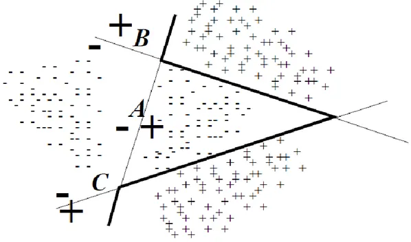
In the following figure, an ensemble of linear classifiers is illustrated. Each line A, B, and C correspond to a linear classifier. The boldface line illustrates the ensemble that classifies new examples with the help of the majority vote of A, B, and C.
25 13 25 06 . 0 ) 1 ( 25 ) 13 ( i i i i X P 21
Figure 4.2 An ensemble of linear classifiers (Oza, 2009)
In order to depict a more accurate picture of a situation, consulting a group of experts is better than consulting just one expert in terms of solving everyday problems. For instance, a patient has a set of symptoms and instead of consulting just one doctor; he/she decides to consult a few doctors in order to make sure about his/her illness. Consulting many doctors, and then based on their diagnosis, he/she can get a fairly accurate idea of the diagnosis. In this example, doctors can be considered as classifiers by analogy. Combining conjectures and judgments of a group of experts lead to more accurate decision when compared to consulting just one expert. As Lyle (2007) points out, if multiple base classifiers are combined, it has often been found that the group is more accurate than the individual, though improvement is not guaranteed.
For this thesis, general ensemble learning methods namely bagging and boosting and RF are used expecting to produce more accurate predictions when compared to the predictions produced by the base classifiers.
22 Bagging
Bagging (Breiman 1996) is an ensemble learning method whose name is derived from bootstrap aggregation. Bagging is a kind of meta-algorithm and it is a special case of model averaging. It is originally designed for classification and usually applied to decision tree models (Sewell, 2008). Bagging makes use of multiple versions of a training set by using the bootstrap namely sampling with replacement. In order to train a different model, each of these data sets is used. The outputs of the models are combined by averaging (in case of regression) or voting (in case of classification) to create a single output. Bagging is easy to implement amongst the ensemble learning methods. It is the simplest method used to improve the performance of a classifier. This method is developed by Leo Breiman (1996) and it is based on aggregating classifiers in order to increase predictive accuracy. Basic idea of bagging is producing different versions of the same classifier using the same training data set. In order to do this, examples are chosen randomly with replacement. It may cause that some examples may be repeated or left out of a training set. As a result of this phase, classifiers are created using the same training sample. The next phase is established by combining all the predictions of each individual classifier to create a final prediction. The final prediction is usually obtained by voting method. The average of all the predictions is performed in this way.
The algorithms for bagging and sampling with replacement are given in figure 4.3. In these algorithms, T is the original training set of N examples, M is the number of base models to be learned, Lb is the base model learning algorithm, the hi’s are the base models, random_integer (a, b) is a function that returns each of the integers from a to b with equal probability, and I (A) is the indicator function that returns 1 if A is true and 0 otherwise (Oza, 2009). In order to create a bootstrap training set from an original training set of size N, we perform N Multinomial trials, where in each trial; we draw one of the N examples. For each trial, each example has probability 1/N of being drawn. The part of the algorithm shown in figure 4.1.1 does exactly this; for N times, the algorithm chooses a number r from 1 to N and adds the rth training example to the bootstrap training set S. Clearly, some of the original training examples will not be selected for inclusion in the bootstrap training set and others will be chosen one time or more (Oza, 2009).
23 Boosting
Boosting (Schapire 1990) is a kind of meta-algorithm which can be received as a model averaging method. It is the most widely used ensemble method amongst the other ensemble methods. Initially a weak classifier is created that it suffices that its accuracy on the training set is only slightly better than a random guessing (Sewell, 2008). A succession of models is built in an iterative fashion. Each of them is trained on a data set in which points misclassified by the previous model are assigned more weight. Eventually, all of the successive models are weighted based on their success. The outputs are combined by making use of voting for classification. This method was developed by Freund and Schapire (1996) as a way of iteratively creating models which complement those that have been created previously (Lyle, 2007). Boosting has common features with bagging that it uses only one type of base classifier, on the other hand, instead of relying on a uniform randomly selected training sets of classifiers, the training sets are based on the strengths and weaknesses of the previously created classifiers. The fundamental difference between bagging and boosting is the addition of a weight to each of the examples in the training set. At the
Figure 4.3 An ensemble of linear classifiers (Oza, 2009)
24
beginning all the weights are set to one, in this way each training example is given equal importance to begin with. At this point it is time to generate the first classifier.
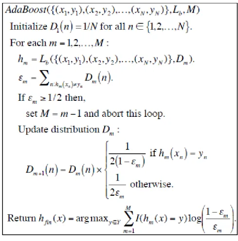
Figure 4.4 AdaBoost Algorithm
The AdaBoost algorithm is illustrated in Figure 4.4. The inputs of the algorithm are a set of N training examples, a base model learning algorithm Lb, and the number M of base models that we want to combine. AdaBoost is originally designed for two-class classification problems, although it is generally used with a large number of classes. This description is based on the assumption that there are two classes. The first phase in AdaBoost is to construct an initial distribution of weights D1 over the training set. This distribution assigns equal weight to all N training examples. Now the loop of the algorithm starts. In order to produce the first base model, we call Lb with distribution D1 over the training set i. After getting back a model h1, we calculate its error ε1 on the training set itself, which is just the sum of the weights of the training examples that h1 classifies incorrectly (Oza, 2009). We
25
require that ε1 < 1/2 which is the weak learning assumption that the error should be less than what we would achieve through random guessing I. In case this condition is not satisfied, then we stop and return the ensemble consisting of the previously-created base models. If this condition is satisfied, then we calculate a new distribution D2 over the training examples as follows. Examples that were correctly classified by h1 have their weights multiplied by 1/(2(1-ε1)). Examples that were misclassified by h1 have their weights multiplied by 1/(2ε1). Because of our condition ε1 < 1/2, correctly classified examples have their weights reduced and misclassified examples have their weights increased. Specifically, examples that h1 misclassified have their total weight increased to 1/2 under D2 and examples that h1 correctly classified have their total weight decreased to 1/2 under D2. After that we go into the next iteration of the loop to construct base model h2 using the training set and the new distribution D2. The key is that the next base model will be created by a weak learner; therefore, at least some of the examples misclassified by the previous base model will have to be correctly classified by the current base model. In this way, boosting forces subsequent base models to correct the mistakes that are made by the previous models. M base models are produced. The ensemble returned by AdaBoost is a function that takes a new example as input and returns the class that gets the maximum weighted vote over the M base models, where each base model's weight is log((1-εm)/εm), which is proportional to the base model's accuracy on the weighted training set presented to it (Oza, 2009).
Random Forest
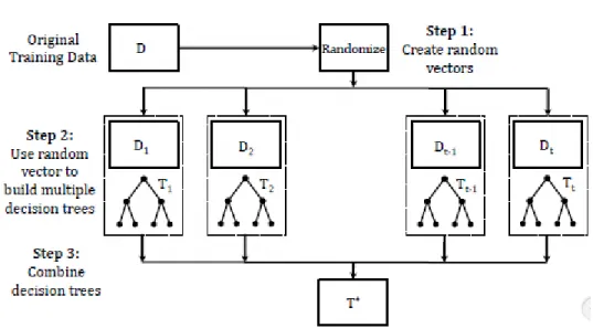
Random Forest is a class of ensemble methods especially designed for decision tree classifiers. The logic behind its structure is that it combines predictions made by many decision trees. In a random forest algorithm, each tree is produced based on a bootstrap sample and the values of a distinct set of random vectors. The random vectors are produced based on a fixed probability distribution. The structure of generating a random forest is based on sampling a dataset with replacement, then selecting m variables from p variables randomly and creating a tree in this way, after creating more trees by repeating the same procedures, the results are combined eventually. Fig 4.3.1 shows the structure of random forests.
26
27
5 IMPLEMENTATION
Dataset Description
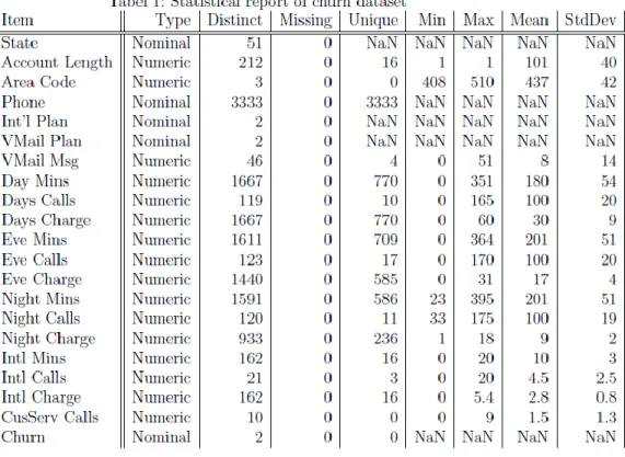
This study is performed on the telco dataset. It is a customer database from University of California, Department of Information and Computer Science, Irvine, CA. The dataset contains historical records of customer churn. There are 3332 instances within dataset with 21 attributes for each customer. Churn is the output variable having the value of either true or false. For each customer record, we can find out information about their corresponding inbound/outbound calls count, inbound/outbound SMS count, and voice mail. In the following table, statistical report of the churn dataset is illustrated in detail. By investigating this dataset, it can be observed that this dataset is a complete dataset with no missing values.
28 Dataset Variables Selection
Full dataset includes 21 variables, but the variables including State, Area Code, and Phone do not contain relevant information that can be used for prediction. In that case we have reduced the number of predictors from 21 to 18. The target variable is Churn which has two values, one of them for each customer: yes or no, telling if a customer is a churner or not. It is only useful for identification purposes.
According to Rulex (Rulex, Inc., 2014) model, the number of variables reduces to 11 variables out of 21. Another study also suggests reducing the number of variables to 11 variables out of 21 as shown in Figure 5.2. The only difference with the Rulex model is that Rulex includes Account Length variable, whereas this study includes State variable. When our algorithms are applied on both of these reduced datasets, the Rulex model generated more efficient results, as a result the Rulex model is chosen as the reduced dataset.
In this thesis, bagging, boosting, and random forest ensemble methods are applied to the datasets that are described above. These algorithms are considered for telecom customer churn classification. In order to perform this study, bagging, boosting, and random forest ensemble methods and decision trees algorithms as base classifiers are used and their results are compared with each other in terms of major performance criteria. Throughout this thesis, decision stump is referred as a weak learner as the base of bagging and boosting ensemble methods. Since it is a weak learner and reducing the number of attributes does not affect its accuracy results, it is only implemented on the full dataset. The classification task comprises of predicting churn based on customer behaviors. Since for many companies, revealing reasons of losing customers, evaluating customer loyalty, taking preventions not to lose customers and developing strategies to regain the customers who churned have become very critical issues.
29
Figure 5.2 Final optimal subset of features (Kozielski et al., 2015)
Throughout this thesis, within WEKA software tool decision stump and J48 base classifiers are implemented purely and they are used as base classifiers for bagging and boosting ensemble methods. Each method is applied on the full dataset with 18 variables and on the reduced dataset with 11 selected variables Rulex (Rulex, Inc., 2014) model.
30 6 Experimental Results
In this section, Decision Stump and J48 Decision Tree classification results are presented first and then the results of the ensemble methods including bagging, boosting and Random Forest are presented. Numerical outputs involving accuracy measures as well as graphical ROC curve outputs are analysed by considering the full and reduced feature sets.
A common method of error rate prediction of a learning algorithm is using stratified tenfold cross-validation. According to this test option in Weka, the dataset is divided into 10 parts initially. These parts comprise of samples which represent approximately the same proportions of the original dataset (Witten et al., 2011). Each part is used in turn for testing while the other parts are used for training. Eventually, the average of the error rates for 10 runs is estimated. For all of our experiments within this study, tenfold cross-validation strategy is applied.
Base Classifiers: Decision Stump and J48 Implementation Decision Stump for Full Data Set
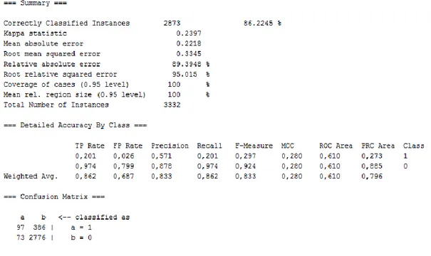
Weka output of the Decision Stump algorithm results with statistical values are presented in Figure 6.1 and Figure 6.2. The figures include prediction errors, accuracy metrics, confusion matrix and areas under the ROC curves for both classes. Weighted averages of accuracy values are also available from the output of this algorithm.
31
Figure 6.1 Weka Output of Decision Stump Algorithm on the Full Dataset
As explained before, Decision Stump is a weak learner for this kind of problems. We use it here for comparison with the other more powerful classification methods. The results in Figure 6.1 are consistent with expectations from a weak learner in that they represent very low TP rate (0,201) in churn group and very high FP rate (0,799) in non-churn group. The MCC value (0.28) and ROC area value (0,61) are also low. For more succesful classifiers both of these values should be closer to their maximal values of 100%.
32
J48 Decision Tree for Full Dataset
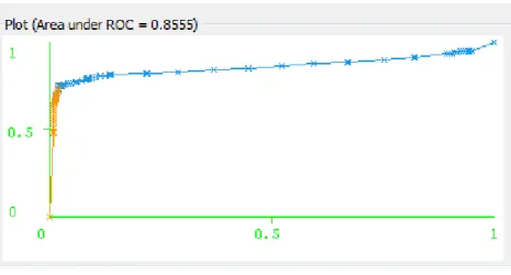
J48 Decision Trees which have good classification properties for most data types. It is also expected to give better results for telecom churn data. The Weka output for J48 implementation and ROC curve are presented in Figure 6.3 and Figure 6.4.
Figure 6.3 Weka Output of J48 Algorithm on the Full Dataset
33
As can be seen from Figure 6.4 TP rate, for the churn group has increased to 0.73 and FP rate has decreased to 0.02. These rates and overall correct classification rate have also improved considerably for the non-churn group. The correct classification rate 0.943 is a high value for this dataset. These results are also reflected in higher MCC (0.758) and ROC area (0.855) values. These and other performance measures display the superiority of J48 based classification over simple Decision Stumps.
Similar results have also been obtained for the reduced data implementation. These results indicate that feature selection successfully reduced the dataset size with almost no loss in accuracy metrics of the J48 Classifier.
34
Implementation Results of Bagging Ensemble Classification
As the first example of ensemble classification, implementation results for bagging are presented, using Decision Stump and J48 as base classifiers both on full and reduced datasets.
6.2.1 Bagging-Decision Stump Base-Full Dataset
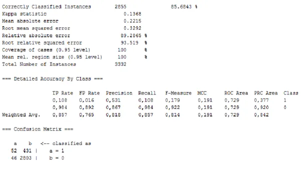
The Weka output for the full data set and the ROC curve are presented in Figure 6.5 and Figure 6.6. Decision Stump is used as a weak base learner for the bagging ensemble classification.
35
Figure 6.6 ROC Curve of Bagging Decision Stump Base on the Full Dataset
The accuracy values in Figure 6.5 do not show any improvements in comparison with simple Decision Stump classification. Some of the results including FP and TP ratios for both classes are even worse than simple Decision Stump implementation. As the Figure 6.6 indicates, the only improvement is in the area under ROC curve which has increased from 0.61 to 0.73. The results indicate that Decision Stump is not a good choice as the base learner for this kind of bagging ensemble classifier formation.
36
6.2.2 Bagging-J48 Decision Tree Base-Full Dataset
Figure 6.7 Weka Output of Bagging J48 Base on the Full Dataset
Figure 6.8 ROC Curve of Bagging J48 Base on the Full Dataset
The results in Figure 6.7 and Figure 6.8 show some improvements in performance values in comparison with simple J48 implementation. The TP and FP rates are better as well as MCC ad ROC area values in bagging ensemble implementation. The ROC area for example increased from 0.855 to 0.913. These results indicate that, even though moderate, improvements are possible in
37
classification performance values when bagging is implemented with a reasonably good learner like J48.
6.2.3 Reduced Dataset Bagging-J48 Decision Tree Base
Figure 6.9 Weka Output of Bagging J48 Base on the Reduced Dataset
Figure 6.10 ROC Curve of Bagging J48 Base on the Reduced Dataset
The results in Figure 6.9 And Figure 6.10 show that the performance value results are essentially similar to the full data set results in that, there have been slight reductions in TP rates and increases in FP rates. The overall performance criteria like F measure, MCC and ROC area also show somewhat negligible reductions.
38
Implementation Results of Boosting Ensemble Classification
In this section, the results for Boosting Ensemble classification are presented for Decision Stump and J48 as base learners. The implementations are performed using Weka Adaboost algorithm.
Boosting-Decision Stump Base-Full Dataset
39
Figure 6.12 ROC Curve of Boosting Decision Stump Base on the Full Dataset
It can be seen from the results in Figure 6.11 and Figure 6.12 that, Decision Stump is not a good choice as a base learner for boosting ensemble classification. Because performance values, although better than simple Decision Stump implementation, are worse than simple J48 and bagging results. Especially, very low MCC values (0.334) and relatively low ROC area value (0.84) and higher accuracy related errors support this claim.
40
Boosting-J48 Decision Tree Base-Full Dataset
Figure 6.13 Weka Output of Boosting J48 Base on the Full Dataset
Figure 6.14 ROC Curve of Boosting J48 Base on the Full Dataset
The results in Figure 6.13 and Figure 6.14 show considerable improvements in all performance measures in comparison with simple and Decision Stump base implementation. It is also possible to conclude that, in general, bagging and boosting classification results are comparable for J48 base implementation. The accuracy values, ROC area and MCC are very close in both cases.
41
Reduced Dataset Boosting-J48 Decision Tree Base
Figure 6.15 Weka Output of Boosting J48 Base on the Reduced Dataset
Figure 6.16 ROC Curve of Boosting J48 Base on the Reduced Dataset
The results in Figure 6.15 and Figure 6.16 show that the accuracy values and other statistics are very close to the full dataset results. Consistent with the previous results, we can conclude that feature selection is an effective data reduction method and should be attempted in ensemble churn analysis.
42
Implementation Results of Random Forest Ensemble Classification Random Forest is a similar ensemble classification method to bagging and boosting. Therefore, its performance results are expected to be close to the other methods we have considered.
6.4.1 Random Forest Classification for Full Dataset
43
Figure 6.18 ROC Curve of Random Forest on the Full Dataset
Figure 6.17 and Figure 6.18 display similar results of performance measures to bagging and boosting with J48 as base learner. With all these ensemble classification methods we obtain MCC values close to 80% and ROC areas close to 91%. The results obtained by such methods are accepted to be fairly good for the classification problem in this study.
6.4.2 Random Forest Classification for Reduced Dataset
44
Figure 6.20 ROC Curve of Random Forest on the Reduced Dataset
Similar to the previous results, performance measure values in the reduced dataset are close to those obtained for the full dataset in case of random forest classification. This finding demonstrates again the importance of dataset size reduction by feature selection.
45
7 Evaluation of the Ensemble Classification Methods Based on Weighted Performance Values
Accuracy Measures
The performance comparisons in this section are all based on the weighted average values of the accuracy measures. The accuracy measures that are summarized in the tables are as follows: Percentage of correctly classified instances, percentage of incorrectly classified instances, true positive rate, F Measure, precision, ROC Area MCC and Kappa Statistic. Precision can be described as the proportion of churn cases in the results amongst all cases. F Measure is a way of combining recall and precision values into a single performance measure. ROC Area is a way of plotting same information in a normalized form. Kappa Statistic is a measure of agreement between observed and predicted classes.
46
7.1.1 Decision Stump Base Implementation Accuracy Results Comparisons
Table 7.1 Accuracy Results Comparisons for Decision Stump Base Implementation
DecisionStump (%values) Bagging (% values) Boosting (% values) Correctly Classified 86,22 85,68 86,85 Incorrectly Classified 13,78 14,32 13,15 TP Rate 86,2 85,7 86,9 Precision 83,3 81,8 84,5 F Measure 83,3 81,4 84,4 ROC Area 61,0 72,9 84,0 Kappa Statistics 23,97 13,68 29,68 MCC 28,0 19,1 33,4