Operating frequency estimation of slot antenna by using adapted kNN algorithm

(1)

International Journal of

Intelligent Systems and

Applications in Engineering

Advanced Technology and Science

ISSN:2147-67992147-6799_{www.atscience.org/IJISAE} Original Research Paper

This journal is © Advanced Technology & Science IJISAE, 2018, 6(1), 29–32 | 29

Operating Frequency Estimation of Slot Antenna by Using Adapted

kNN Algorithm

Enes Yigit

1 *

Accepted : 16/11/2017 Published: 30/03/2018 DOI: 10.1039/b000000x

Abstract: In this study ultra-high frequency slot antenna’s operating frequency is estimated by using adapted k-nearest neighbor (kNN) algorithm. kNN doesn’t use the training data points to do any generalization and it can be usually used for many classification. However, kNN can be adapted to estimate slot antenna’s operating frequency by assessing the best k-nearest value. To find the optimal k for operating frequency estimation, 96 slot antennas with seven antenna parameters are simulated with respect to the operating frequency by using a computational electromagnetic software. Antenna parameters includes the patch dimensions, height and relative permittivity of the substrate. The simulated 81 antennas are used to construct feature data pool and the residual 15 antennas are used to test kNN algorithm. The performance of the kNN is evaluated by comparing the output of operating frequency to the simulated one. Then the proposed model is corroborated with simulated antennas and validating with prototyped antenna data. The results shows that the kNN based model simply and fast computes the operating frequency of the slot antennas much close to real one without performing any simulations or measurement. Keywords: Slot antenna, antenna analysis, operating frequency, kNN algorithm

1. Introduction

Slot antennas are the microwave antennas in which the radiation patterns are determined by the size and shape of a slot in a radiating surface. Slot loading technique are commonly used to form little patch antennas, suitable for modern wireless technologies. Therefore the miniaturization in size and tuning the operating frequency for slot antennas have become popular [1-9]. In literature there can be found different shaped slot antennas such as rectangular ring [1], L [2], C [3] and E [4] shapes. While this type of antennas are commonly loaded in symmetrical with respect to the edge of the patch, slot antennas are constituted by asymmetrical notching one side of the patch [5]. For this reason, slot antennas needs great effort for analysis, like cavity model [6] and transmission line model [7] because of its irregular shapes. In general, these techniques [6, 7] could not be employed to analysis the slot antennas alone. On the other hand, thanks to computer-based software combined with computational electromagnetic (CEM) [8], the slot antennas can be simulated and analyzed by using very expensive CEM-based simulation tools experience. In order to find the alternative techniques of simply analyzing the slot antennas, (particularly operating frequency determination) artificial intelligence systems have used recently [9-13]. These techniques usually need training and generalization procedure to make best estimation. On the other hand, k-nearest neighbor (kNN) doesn’t need to use the training data points to do any generalization so it can be easily used for many categorizations or classification [14-16]. Although kNN is the simplest controlled learning algorithm, it hasn’t been used to estimate operating frequency of the antennas so far. In this study kNN is adapted to estimate the operating frequency of the slot antenna. For this purpose, the performance of the kNN algorithm is defined to find best k value

that gives the minimum error between target and output. In kNN algorithm, the relations between the features of the input parameters can be defined by using different distance metric. In this study, Euclidean distance metric is used to estimate the operating frequency of the designed antenna with six physical parameters and a relative permittivity of the substrate. In order to generate the feature data and estimate the best k value, 96 slot antenna with different parameters are simulated in terms of operating frequency by using a CEM software. The simulated data of 81 antenna is used to generate feature data and the 15 are utilized to test the accuracy. After using kNN algorithm, for k=1 the 15 testing data is estimated with mean absolute error (MAE) of 0.019. Then the proposed estimator is validated using constructed slot antenna prototyped.

2. k-Nearest Neighbor Algorithm

kNN is the simplest controlled learning algorithm among the whole machine learning algorithms [14]. It doesn’t use the training data points to do any generalization so it is also called a lazy algorithm. In order to apply kNN algorithm, feature vectors in a multidimensional feature space have to be created. Thus, the desired test object can be defined according to distance to the nearest neighbor feature. The frequently used distance metric for variables is Euclidean distance and number of the neighbor objects is defined by k coefficient. In the chosen k-nearest neighborhood, the query object is appointed to class of the most uncategorized data. For example, the test sample (red square) given in Fig.1 should be classified either to the yellow spheres or to the black stars. If k value is chosen as four (dashed line) query object is assigned to the yellow sphere because there are 3 yellow spheres and only 1 black star inside the inner dashed circle. If k is chosen as seven (solid line circle) it is assigned to the second class because there are four black star inside the inner circle. So, the query object can be defined with respect to k value. However, if we need to make estimation instead of classification, we have to re-define

_______________________________________________________________________________________________________________________________________________________________________________________________________________________________________________________________________________________________________________________________

1_{Department of Electrical and Electronics Engineering,}

Engineering Faculty, Karamanoglu Mehmetbey University, 70100, Karaman, Turkey

(2)

query object appointment as given in section 3.2 in detail.

?

Fig. 1. Demonstration of KNN detection

3. Design of slot antenna and query object

appointment

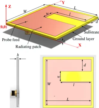
The constructed slot antenna’s geometry is illustrated in Fig.2. The length and width of antenna is identified as 𝐿 𝑎𝑛𝑑 𝑊 respectively.

It consists of ground layer, substrate with ℎ thickness and

𝜀𝑟 relative permittivity. The probe feed is positioned at(𝑥0, 𝑦0).

The dimensions of the rectangular slot is defined with 𝑙 𝑎𝑛𝑑 𝑤 and shifted as 𝑑 from the upper side as seen in Fig.2. To determine the operating frequency of the designed slot antenna, 7 parameters are simulated and used as input feature data of the kNN model. The kNN feature data pool is constructed with 81 antenna data and then for each test (query) object the nearest neighborhood relations calculated for different k values. The objective of the kNN algorithm is to find best k coefficient which gives the minimum MAE between the target and output.

l w W L d h Probe feed Radiating patch Substrate Ground layer X Z Y (0,0) h d w W L l

Fig. 2. Three dimensional representation of the designed slot antenna 3.1. Simulations

In order to be used for ultra-high frequency (UHF) band applications, the antennas’ parameters are determined so that they operate between 1.15 GHz and 3.35 GHz. 96 different antennas are simulated by means of CEM software HyperLynx® 3D EM [17]

running method of moment and all parameters are given in Table 1. To make a uniformly distributed data pool, the outer sizes of the slot antennas are selected in three groups. Each groups has 32 antenna and outer dimensions of groups are 30, 20; 40, 30 and 50,

40 including different parameters of 𝑙, 𝑤, 𝑑, ℎ and relative

permittivity 𝜀𝑟. The antennas source coordinates are defined as

𝑥0= 5𝑚𝑚 , 𝑦0= 5𝑚𝑚 and 1 volt wave source is used to feed

them. Simulations are realized between 1 to 5 GHz for a total of 81 discrete points.

Table 1: Simulated slot antenna parameters Patch dimensions (mm) 𝒉 𝒎𝒎 𝜺𝒓 𝑳 𝑊 𝑙 𝑤 𝑑 30 20 10;20 5;10 3;6 1.6; 2.5 2.33; 4.4 40 30 15;30 7.5;15 5;10 50 40 20;40 10;20 7;14 3.2. Adapted kNN Algorithm

At the end of the 96 simulation, the simulated data of 81 antenna is used to generate feature data pool and the 15 are utilized to test the accuracy. To create feature vector the 81 antennas are located with respect to multidimensional distance to origin as given equation 1.

𝑑0𝑎= √𝐿𝑎2+ 𝑊𝑎2+ 𝑙𝑎2+ 𝑤𝑎2+ 𝑑𝑎2+ ℎ𝑎2+ 𝜀𝑟 𝑎2 (1)

where 𝑑0𝑎 is the Euclidian distance vector of each test antenna with

respect to origin (0, 0). In Eq.1, 𝑎 = 1 𝑡𝑜 81 indicates the each

antenna and each 𝑑0𝑎≡ 𝑑𝑓𝑎 correspond to operating

frequency 𝑑𝑓𝑎, which is obtained by simulations. In order to find

test antennas operating frequency, the distances from each test

antennas to each 𝑑0𝑎 is obtained by using Eq. 2.

𝑑𝑡𝑎= √

(𝐿𝑎− 𝐿𝑡)2+ (𝑊𝑎− 𝑊𝑡)2+

(𝑙𝑎− 𝑙𝑡)2+ (𝑤𝑎− 𝑤𝑡)2+

(𝑑𝑎− 𝑑𝑡)2+ (ℎ𝑎− ℎ𝑡)2+ (𝜀𝑟 𝑎− 𝜀𝑟 𝑡)2

(2)

In Eq. 2, 𝑡 indicates the query antenna and 𝑑𝑡𝑎 is the 1 × 𝑎 sized

distance vector. To find nearest neighborhood, 𝑑𝑡𝑎 vector is

reordered from minimum (nearest) to maximum (farthest) and

corresponding operating frequencies are defined as 𝑑𝑡𝑓𝑚. By

using 𝑑𝑡𝑓𝑚, different neighborhood values can be calculated with

respect to 𝑚 value. In this study 𝑚 is scanned between 1 𝑡𝑜 𝑘 =

10 and the query objects (𝑞𝑜𝑡𝑘) are appointed regarding to 𝑘, as

given in Eq. 3.

𝑞𝑜𝑡𝑘=

∑𝑘𝑚=1𝑑𝑡𝑓𝑚

𝑘 (3)

where 𝑞𝑜𝑡𝑘 is the appointed operating frequency vector regarding

to 𝑘 value. After determining the 𝑞𝑜𝑡𝑘 for each k, the absolute error

(AE) is calculated as given below;

𝐴𝐸𝑡𝑘= 𝑞𝑜𝑡𝑘− 𝑜𝑓𝑡 (4)

where 𝑜𝑓𝑡 is the operating frequency of 𝑡’ 𝑡ℎ test antenna derived

by simulation. The MAE is calculated by taking average value of the whole query objects as given

𝑀𝐴𝐸𝑘=

∑𝑁𝑡=1𝐴𝐸𝑡𝑘

𝑁 (5)

where N is the number of the test objects. For different k values MAE are compared among to each other and the minimum MAE is found with respect to k. Hence, the operating frequency determination algorithm is concluded, with the help of estimated k value.

(3)

4. Testing the kNN algorithm

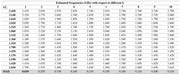
The accuracy of the algorithm is tested through 15 slot antennas data that is not utilized in feature matrix. Parameters of 15 simulated antennas with respective operating frequency values are given in Table 2. These test antennas are then used for query object in kNN algorithm. The k value is changed from 1 to 10 and Eq. 3 is calculated for each k value and test antenna. The estimated operating frequencies of the query antennas for different k values along with MAE results are given in Table 3. The best estimation result is obtained for k=1 with MAE of 0.019.

Table 2: Simulated Test antennas parameters

Patch dimensions Operating Frequency t 𝑳 𝑾 𝒍 𝒘 𝒅 𝒉 𝜺𝒓 𝒐𝒇𝒕 (GHz) 1 30 20 10 5 3 2.5 4.4 2.426 2 30 20 10 10 6 2.5 2.33 3.140 3 30 20 20 5 3 1.6 4.4 1.611 4 30 20 20 5 6 1.6 2.33 2.015 5 30 20 20 10 6 1.6 4.4 1.512 6 40 30 15 7.5 5 1.6 4.4 1.860 7 40 30 15 15 5 2.5 2.33 2.107 8 40 30 30 7.5 5 1.6 2.33 1.357 9 40 30 30 7.5 10 2.5 2.33 1.311 10 40 30 30 15 5 2.5 4.4 1.695 11 50 40 20 10 7 1.6 4.4 1.466 12 50 40 20 10 14 2.5 4.4 1.174 13 50 40 20 20 14 1.6 2.33 1.585 14 50 40 40 10 7 2.5 4.4 1.421 15 50 40 40 20 7 2.5 2.33 1.814

5. Validating the estimator

To test and validate the proposed model’s performance, the slot

antenna is printed on a 25x35 mm2_{FR4 PCB substrate as seen in}

Fig. 3. The dielectric permittivity, tangent loss and thickness of the PCB are 4.4, 0.02 and 2.5 mm, respectively. The prototyped antenna of which parameters given in Table 4 is measured by the help of Keysight N5224A PNA network analyzer. The measured

S11 parameter is shown in Fig.4 in comparison with the simulated

one.

(a)

(b)

Fig. 3. The scene of prototyped slot antenna (a) front view, (b) back view with reference coin

Table 3: The estimated operating frequencies of the simulated antennas for different k values

Estimated frequencies (GHz) with respect to different k

𝒐𝒇𝒕 1 2 3 4 5 6 7 8 9 10 2.430 2.410 2.830 2.970 2.830 2.740 2.810 2.740 2.700 2.740 2.780 3.140 3.150 2.770 2.640 2.760 2.830 2.760 2.700 2.760 2.720 2.680 1.610 1.630 1.870 1.960 1.850 1.790 1.840 1.790 1.760 1.790 1.820 2.020 2.050 1.790 1.710 1.810 1.880 1.840 1.860 1.880 1.840 1.860 1.510 1.540 1.770 1.860 1.780 1.730 1.780 1.820 1.780 1.760 1.790 1.860 1.870 2.220 2.330 2.130 2.030 2.040 2.040 1.990 1.940 1.960 2.110 2.100 1.840 1.750 1.840 1.900 1.850 1.810 1.900 1.980 1.960 1.360 1.380 1.570 1.640 1.550 1.590 1.620 1.580 1.540 1.560 1.530 1.310 1.280 1.530 1.610 1.550 1.600 1.620 1.580 1.550 1.560 1.580 1.700 1.670 1.490 1.430 1.500 1.540 1.500 1.470 1.510 1.540 1.520 1.470 1.490 1.560 1.590 1.480 1.500 1.510 1.460 1.430 1.440 1.450 1.170 1.160 1.360 1.420 1.440 1.480 1.510 1.460 1.430 1.450 1.420 1.590 1.600 1.390 1.320 1.380 1.420 1.380 1.350 1.380 1.400 1.370 1.420 1.410 1.670 1.740 1.660 1.610 1.660 1.700 1.650 1.620 1.630 1.810 1.790 1.570 1.490 1.580 1.640 1.590 1.560 1.600 1.630 1.610 MAE 0.019 0.250 0.330 0.240 0.210 0.250 0.240 0.210 0.200 0.210

Table 4. The measured and estimated operating frequencies of the prototyped slot antenna

Antenna Parameters Patch dimensions (mm) 𝒉 𝜺𝒓 𝑳 𝑾 𝒍 𝒘 𝒅 30 20 10 5 3 3 4

Operating Frequency Absolute error

f simulation f measurement f estimated AE simulation AE measurement 2.426 2.430 2.409 0.017 0.021 2.3 2.35 2.4 2.45 2.5 -20 -15 -10 -5 0 X axes: Frequency (GHz) Y axe s :dB Simulation Measurement X: 2.426 GHz Y: -17.5 dB X: 2.43 GHz Y: -13.5 dB

(4)

It can clearly be comprehended from Fig.4 and Table 4 that, the estimated and measured operating frequencies are much close to simulated results. Thus, kNN based model can be effectively handled to compute the operating frequency of the slot antennas

without solving complex mathematical functions and

transformations. Additionally, the proposed kNN algorithm can be enhanced to handle similar tasks of nonlinear electromagnetic problems.

6. Conclusion

In this paper, kNN based estimator is implemented to finding the operating frequencies of the slot antennas. In order to make accurate estimation, the number of k neighborhood is varied for a total of 10 different distance metric. The feature matrix is constituted with 81 slot antennas having various physical and electrical parameters is simulated with the help of HyperLynx® 3D EM in terms of the operating frequency. In kNN model, 15 antennas are used as a query object for testing the best K estimation. The performance of the kNN is evaluated by comparing the appointed operating frequency to the simulated one. Then the proposed estimator is corroborated with simulated antennas and validated with prototyped antenna data. The results shows that the best estimation is occurred for k=1. Once the best k value is properly found, the operating frequency of patch antennas can be accurately computed.

References

[1] A. A. Deshmukh and G. Kumar, “Formulation of resonant frequency for compact rectangular microstrip antennas,” Microw. Opt. Techn. Let., vol. 49, pp. 498-501, 2007.

[2] Z. N. Chen, “Radiation pattern of a probe fed L-shaped plate antenna,” Microw. Opt. Techn. Let., vol. 27, pp. 410-413, 2000.

[3] A. Akdagli, A. Kayabasi and I Develi, “Computing resonant frequency of C-shaped compact microstrip antennas by using ANFIS,” Int. J. Elec., vol. 102, pp. 407-417, 2015.

[4] A. Toktas and A. Akdagli, “Computation of resonant frequency of E-shaped compact microstrip antennas,” J. Fac. Eng. Arch. Gazi Univ., vol. 27, pp. 847-854, 2012.

[5] S. Bhunia, “Effects of slot loading on microstrip patch antennas”, International journal of wired and wireless communications, vol. 1, pp. 1-6, 2012.

[6] W. F. Richards, Y. T. Lo and D. D. Harrisson, “An improved theory for microstrip antennas and applications,” IEEE T. Anten. Propag., vol. 29, pp. 38-46, 1981.

[7] K. Bhattacharyya and R. Garg, “A generalized transmission line model for microstrip patches,” IEE PROC-H., vol. 132, pp. 93-98, 1985.

[8] D. B. Davidson, Computational electromagnetics for RF and microwave engineering, Cambridge University Press, Cambridge, United Kingdom.2005.

[9] A. Akdagli, A. Toktas, M. B. Bicer, A. Kayabasi, D. Ustun and K. Kurt, “ANFIS model for determining resonant frequency of rectangular ring compact microstrip antennas,” Int. J. Appl. Electrom., vol. 46, pp. 483-490, 2014.

[10] K. Guney and N. Sarikaya, “Adaptive neuro-fuzzy inference system for computing the resonant frequency of circular microstrip antennas,” The Applied Computational Electromagnetic Society, vol. 19, pp. 188-197, 2004.

[11] F. Güneş, N. T. Tokan and F. Gürgen, “A consensual modeling of the expert systems applied to microwave devices,” International Journal of RF and Microwave computer-Aided Engineering, vol. 20, pp. 430-440, 2010.

[12] Y. Tighilt, F. Bouttout and A. Khellaf, “Modeling and design of

printed antennas using neural networks,” International Journal of RF and Microwave Computer-Aided Engineering, vol. 21, pp. 228-233, 2011.

[13] A. R. Venmathi and L. Vanitha, “Support vector machine for bandwidth analysis of slotted microstrip antenna,” International Journal of Computer Science, Systems Engineering and Information Technology, vol. 4, pp. 67-61, 2011.

[14] K.Sabancı, M. Kokulu, “The Classification of Eye State by Using kNN and MLP Classification Models According to the EEG Signals” International Journal of Intelligent Systems and Applications in Engineering, 3(4), 127-130, 2015

[15] M.F. Unlersen, K. Sabancı “The Classification of Diseased Trees by Using kNN and MLP Classification Models According to the Satellite Imagery” International Journal of Intelligent Systems and Applications in Engineering, 4(2), 25–28, 2016.

[16] K.Sabanci, M. Akkaya, “Classification of Different Wheat Varieties by Using Data Mining Algorithms.” ” International Journal of Intelligent Systems and Applications in Engineering, 4(2), 40–44, 2016.

[17] HyperLynx® 3D EM, Version 15, Mentor Graphics Corporation, 8005 SW Boeckman Road, Wilsonville, OR 97070.