Selçuk J. Appl. Math. Selçuk Journal of Vol. 5. No. 1. pp. 3-10, 2004 Applied Mathematics
A Note on Non-identi…biality Problem of Finite Mixture Distribution Models in Model-based Classi…cation
Hamza Erol
Çukurova University, Faculty of Arts & Sciences, Department of Statistics 01330 Adana, Turkey;
e-mail: [email protected]
Received: February 2, 2004
Summary. The probability density functions (pdfs) of the mixture distribu-tion models (mdms) for two di¤erent populadistribu-tions can be compared by using a distance function (metric) between them in model-based classi…cation applica-tions. The result of the comparison may not be true if the component densities of the mdms are permutation functions. Thus, non-identi…biality problem of …nite mixture distribution models. In other words, the order of the component densities of the mdms should be taken into account. If the component densi-ties of the mdms are permutation functions then the pdfs of the mdms for two di¤erent population looks like similar but in fact they are completely di¤erent. Such a case may cause wrong inference in the applications in which the mdms used, for example in classi…cation applications. The componentwise distance function is proposed for the comparison of the pdfs of the mdms for two dif-ferent populations if the component densities are permutation functions. The condition under which the value of the distance function between the pdfs of the mdms for two di¤erent populations is equal to the value of the componentwise distance function between the pdfs of the mdms for two di¤erent populations is given.
Key words: Finite mixture distribution model, Hellinger distance, model-based classi…cation, non-identi…biality, permutation functions
2000 Mathematics Subject Classi…cation: 60E05
1. Introduction
Let’s consider two di¤erent populations each consisting of boys and girls. Let’s assume each population has the mixture of two univariate normal distributions
with respect to the variate height in centimeters. This is the most common and well known case in the mixture distribution studies (Everitt and Hand, 1981; Lindsay, 1995).
In some studies the assumption “the components of the pdfs of mdms are arranged, for convenience, according to their means such that their means are in increasing order”is made. This assumption sometimes may be false as explained below and should be checked for validity.
There are two cases that should be considered when the pdfs of the mdms for two di¤erent populations are compared by using a distance function (metric), for instance Hellinger distance function (Beran, 1977; Titterington et al., 1983) between them. Hellinger distance function is preferable as the distance function (metric) since it has well properties in mathematical and statistical sense(Rao, 1995a; Rao, 1995b).
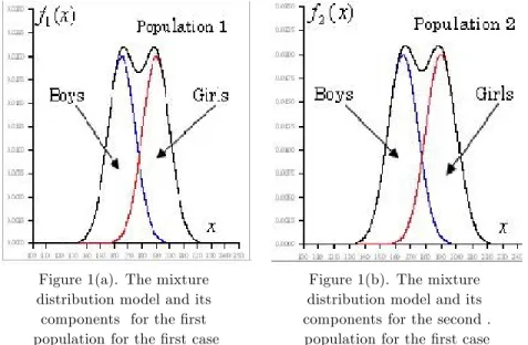
Figure 1(a). The mixture Figure 1(b). The mixture distribution model and its distribution model and its components for the …rst components for the second . population for the …rst case population for the …rst case
Figure 1. The corresponding component densities of the mdms for two di¤erent populations are in the same order with respect to their means. There is no non-identi…biality problem of …nite mixture distribution models in the …rst case.
The …rst case is if the corresponding component densities of both mdms are in the same order with respect to their means then the component densities are in regular order as shown in Figure 1. In this case there is no problem in the comparison of the pdfs of the mdms for two di¤erent populations. They can be compared by using Hellinger distance function between them.
The graphs of the pdfs of the mdms with their component densities for two di¤erent populations, thus, population1 and population 2 for the …rst case is shown in Figure 1(a) and Figure 1(b) respectively. The corresponding compo-nent densities (the compocompo-nent densities for boys and the compocompo-nent densities
for girls) of both mdms are in the same order with respect to their means. So the component densities are in regular order and there is no problem in the comparison of the pdfs of the mdms for two di¤erent populations in this case. They can be compared by using Hellinger distance function between them.
The second case is if the corresponding component densities of both mdms are not in the same order with respect to their means then the component densities are in irregular order as shown in Figure 2 and the component densities of the mdms behave as permutation functions. If the component densities of the mdms are permutation functions then the pdfs of the mdms for two di¤erent population looks like similar but in fact they are completely di¤erent. In this case there is a problem in the comparison of the pdfs of the mdms for two di¤erent populations. They can be compared by using componentwise Hellinger distance function between them to overcome this problem.
Figure 2(a). The mixture Figure 1(b). The mixture distribution model and its distribution model and its components for the …rst components for the second population for the second case population for the second case.
Figure 2. The corresponding component densities of the mdms for two di¤erent populations are in irregular order with respect to their means. There is non-identi…biality problem of …nite mixture distribution models in the second case. The reason for this problem is neither the mixture modelling nor the distance function used. The reason for this problem is the natural structure of the mixture itself. This problem is very important and must be taken into account in the applications such as in classi…cations where the mdms used since it may cause wrong inference in the applications such as in classi…cations where the mdms used.
The graphs of the pdfs of the mdms with their component densities for two di¤erent populations, thus, population1 and population 2 for the second case is shown in Figure 2(a) and Figure 2(b) respectively. The corresponding compo-nent densities (the compocompo-nent densities for boys and the compocompo-nent densities
for girls) of both mdms are not in the same order with respect to their means. So the component densities are in irregular order and there is a problem in the comparison of the pdfs of the mdms for two di¤erent populations in this case since the component densities of the pdfs of the mdms are permutation func-tions. They can be compared by using component Hellinger distance function between them.
2. Method
Let the mixture model for the i th population be the mixture of two univariate normal distributions having the form,
(1) fi(x; i1; i2; i1; i2; pi1) = 2 X j=1 pijfij(x; ij; ij) 1 < x < +1; 1 < ij < +1; ij > 0; 0 < pij < 1
with respect to the variate height for i = 1; 2 and j = 1; 2. The component densities having the form,
(2) fij(x; ij; ij) = 1 p 2 ij exp ( 1 2 (x ij ij 2) 1 < x < +1 1 < ij < +1; ij > 0
Let the …rst component correspond to boys and the second component cor-respond to girls. fi1(x; i1; i1) corresponds to the density for the variate height
of boys and fi2(x; i2; i2) corresponds to the density for the variate height of
girls in the i th population. ij and 2
ij are the j th component mean and
the variance of the i th population respectively. pij’s are mixture proportions
such that
2
P
j=1
pij = 1 for i = 1; 2.
The pdfs of the mdms (fi(x; i1; i2; i1; i2; pi1); i = 1; 2 for two di¤erent
pop-ulations) of the form in equation (1) can be established by using EM algorithm (McLachlan and Krishnan, 1997) or the methods explained by McLachlan and Peel (2000).
There are two cases should be considered:
Case 1: If the corresponding component densities of both mdms are in the same order with respect to their means as shown in Figure 1. Thus, if
for two di¤erent populations then the component densities are in regular order. In this case there is no problem in the comparison of the pdfs of the mdms for two di¤erent populations.
The pdfs of the mdms f1(x; 11; 12; 11; 12; p11) (or in short f1(x)) and
f2(x; 21; 22; 21; 22; p21) (or in short f2(x)) for two di¤erent populations can
be compared by using Hellinger distance function between them. Hellinger distance function between f1(x) and f2(x) is denoted by HDf1;f2 and de…ned
by (4) HDf1;f2 = Z D 1 2 p f1(x) p f2(x) 2 dx D = fx j 1 < x < +1g
Hellinger distance between two pdfs of the mdms is geometrically equal to the area not common under both curves. Hellinger distance takes values between 0 and 2. Thus,
(5) 0 HDf1;f2 2
Case 2: If the corresponding component densities of both mdms are not in the same order with respect to their means as shown in Figure 2. Thus, if
(6) 11< 12 and 21> 22 or 11> 12and 21< 22
then the component densities are in irregular order and the component densities of the mdms behave as permutation functions. In this case there is a problem in the comparison of the pdfs of the mdms for two di¤erent populations. In such a case the mdms of two di¤erent populations look like similar to each other but in fact they are completely di¤erent. The reason for this problem is neither the mixture modeling nor the distance function used.
The reason for this problem is the natural structure of the mixture itself. This problem is very important and must be taken into account in the applica-tions such as in classi…caapplica-tions where the mdms used since it may cause wrong inference in the applications such as in classi…cations where the mdms. In this case the mdms for two di¤erent populations can be compared by using compo-nentwise Hellinger distance function between them to overcome this problem.
The mdms f1( x; 11; 12; 11; 12; p11) ( or in short f1( x ) ) and
f2(x; 21; 22; 21; 22; p21) (or in short f2(x)) for two di¤erent populations can
be compared by using componentwise Hellinger distance function. Compo-nentwise Hellinger distance function between f1(x) and f2(x) is denoted by
(7) CHDf1;f2 = 2 X j=1 Z D 1 2 q p1jf1j(x) q p2jf2j(x) 2! dx D = fx j 1 < x < +1g
The condition under which the value of Hellinger distance function between the pdfs of the mdms is equal to the value of the componentwise Hellinger distance function between the pdfs of the mdms for two di¤erent populations is given by the following Theorem 1.
Theorem 1 The value of Hellinger distance function between the pdfs of the mdms is equal to the value of the componentwise Hellinger distance function between the pdfs of the mdms for two di¤ erent populations if and only if the equality (8) Z D p p11f11(x)p21f21(x)dx + Z D p p12f12(x)p22f22(x)dx Z D p f1f2dx = 0 holds.
Proof. ( The proof will be given only for if part of Theorem 1)
(If part): Starting from the value of Hellinger distance function between the pdfs of the mdms f1(x) and f2(x) we have
(9) HDf1;f2 = Z D p f1(x) p f2(x) 2 dx
as de…ned by the equation (4). The equality in equation (9) can be writen as
(10) HDf1;f2 = Z D f1(x) 2 p f1(x)f2(x) + f2(x) dx
or in terms of component densities as
(11) HDf1;f2 = Z D (p11f11(x) + p22f22(x)) dx + Z D (p12f12(x) + p21f21(x)) dx 2 Z D p f1(x)f2(x) dx
First by adding and subtracting the terms 2pp11 f11 (x) p21 f21(x) and
2pp12f12(x)p22f22(x) in the integral in equation (11) and then making some
arrangements we have (12) HDf1;f2 = Z D (p11f11(x) + p21f21(x)) dx 2 Z D p p11f11(x)p21f21(x) dx + Z D (p12f12(x) + p22f22(x)) dx 2 Z D p p12f12(x)p22f22(x) dx + 2 Z D p p11f11(x)p21f21(x)dx +2 Z D p p12f12(x)p22f22(x)dx 2 Z D p f1(x)f2(x)dx
The …rst two terms in equation (12) are equal to the componentwise Hellinger distance function between the component densities of the pdfs of the mdms for two di¤erent populations. So we have
(13) HDf1;f2= 2 X j=1 Z D q p1jf1j(x) q p2jf2j(x) 2 dx +2 Z D p p11f11(x)p21f21(x)dx + 2 Z D p p12f12(x)p22f22(x)dx 2 Z D p f1(x)f2(x)dx or (14) HDf1;f2 = CHDf1;f2+ 2 Z D p p11f11(x)p21f21(x)dx +2 Z D p p12f12(x)p22f22(x)dx 2 Z D p f1(x)f2(x)dx
The value of Hellinger distance function between the pdfs of the mdms is equal to the value of the componentwise Hellinger distance function between the pdfs of the mdms for two di¤erent populations if the condition in equation (8) holds.
3. Conclusions
In some cases the component densities of the mdms for two di¤erent popula-tions are in irregular order and they behave as permutation funcpopula-tions. In such cases the pdfs of the mdms for two di¤erent population look like similar but in fact they are completely di¤erent. This is non-identi…ability problem of …nite mixture distribution models. The reason for this problem is neither the mix-ture modeling nor the distance function used. The reason for this problem is the natural structure of the mixture itself. This problem is very important and must be taken into account in the applications such as in classi…cations where the mdms used since it may cause wrong inference in the applications such as in classi…cations where the mdms used.
Theorem 1 provides autocontrol whether the component densities of the mdms for two di¤erent populations are in regular order or not. If the component densities of the mdms for two di¤erent populations are in regular order then the value of Hellinger distance function and the value of the componentwise Hellinger distance function are close to each other (or approximately equal to each other) for two di¤erent populations. If the value of Hellinger distance function and the value of the componentwise Hellinger distance function are di¤erent from each other then the component densities of the mdms for two di¤erent populations are in irregular order or the component densities of the mdms for two di¤erent populations are permutation functions. In this case the componentwise Hellinger distance function should be used to compare the pdfs of the mdms for two di¤erent populations.
References
1. Beran, R. (1977): Minimum Hellinger distance estimates for parametric models, The Annals of Statistics, 5(3), 445-467.
2. Everitt, B. S., Hand, D. J. (1981): Finite Mixture Distributions, London, Chapman and Hall.
3. Lindsay, B. G. (1995): Mixture Models: Theory, Geometry and Applications, USA, NSF-CBMS Regional Conference Series in Probability and Statistics, Vol. 5.
4. McLachlan, G. J., Krishnan, T. (1997): The EM Algorithm and Extensions, New York, John Wiley & Sons, Inc.
5. McLachlan, G. J., Peel, D. (2000): Finite Mixture Models, New York, John Wiley & Sons, Inc.
6. Rao, C. R. (1995a): The use of Hellinger Distance in graphical displays of contin-gency table data Multivar Statist., 143-161.
7. Rao, C. R. (1995b): A rewiev of canonical coordinates and an alternative to correspondence analysis using Hellinger Distance. Qüestiió, Vol. 19, issue 1,2,3, 23-63. 8. Titterington, D. M., Smith, A. F. M., Makov, U. E. (1985): Statistical Analysis of Finite Mixture Distributions, Chichester, John Wiley & Sons.