INTERNATIONAL JOURNAL OF AGRICULTURE &BIOLOGY ISSN Print: 1560–8530; ISSN Online: 1814–9596 17–0394/2018/20–5–966–974
DOI: 10.17957/IJAB/15.0584 http://www.fspublishers.org
Full Length Article
Determination of Possibilities of Microwave Application for Weed
Control
Koray Kaçan1*, Engin Çakır2 and İkbal Aygün2
1Plant and Animal Production, Ortaca Vocational School, Muğla Sıtkı Koçman University, Turkey
2Department of Agricultural Engineering and Technologies, Faculty of Agriculture, Ege University, Turkey
*For correspondence: [email protected]
Abstract
Herbicide use is a continuously growing threat against effective implementation of sustainable agriculture potential. Herbicide use for controlling weeds incurs at the cost of environment and is least cost effective. It also leads to herbicide resistance. This study uncovered possibilities of using microwave energy to control weeds in laboratory conditions. Tests were conducted on a prototype of microwave-based weed control. This study found out the limit of power levels for controlling weeds. For microwave experiments, the most important weeds were selected from among the perennial and annual weeds determined in cotton and maize fields. Microwave radiations were applied on annual weeds; black nightshade (Solanum nigrum L.) and common cocklebur (Xanthium strumarium L.) in addition to perennial weeds; Bermuda grass (Cynodon dactylon (L.) Pers.) and Johnson grass (Sorghum halepense (L.) Pers.). The weeds with three different development stages: (BBCH Scale; 12–13, 19–23, 29–33), four leaves, eight leaves and weeds at seeding stage were exposed to minimum 1.6 kW and maximum 5.6 kW microwave power with two different forward feed rates of 0.1–0.3 m s-1. Results showed that microwave power required to
control the weeds increased with increasing the speed of feed rate. The optimum microwave power to control weeds was at a forward speed of 1 m s-1. The ED
50, ED80 and ED90 values were determined according to the dose-response effect analyses for
fresh and dry weights of weeds. Consequently, the control of cocklebur and black nightshade required much less power in comparison to Johnson grass and Bermuda grass. Bermuda grass was the only weed which required maximum energy level at all feed rates at laboratory conditions. © 2018 Friends Science Publishers
Keywords: Microwave; Weed control; Cotton; Maize; Different power levels; Different feed rates
Introduction
The issue that takes the most effort and cost in agricultural practices are weeds. In fact, the yield losses worldwide by weeds are around 10% on average (Oerke, 2006). These losses are about 32% in maize, cotton and some other significant crops. In Turkey, the most important aim of the economy is to achieve the highest agricultural production by minimizing production costs. Especially the loss of yield due to weeds in maize and cotton yield is in the range of 21–61%. Usage of herbicides for a long time in order to reduce these yield losses is raising concerns for their harmful effects on ecology and human health (Bond and Grundy, 2001). Additionally, excessive herbicide usage leads to problems like herbicide resistance and emergence of new invasive species (Owen et al., 2007; Brodie et al., 2009).
As a result of these reasons, demands for non-chemical agricultural practices are increasing, which necessitates sustainable agriculture (Bond and Grundy, 2001). Recently, various non-chemical control methods are being used and these include flame-burning, mulching,
covering, radiation and laser applications. However, the main issues with non-chemical weed control methods are duration of control, insufficient effectiveness and that their control activity is not as effective as the spread of weeds (Beveridge and Naylor, 1999).
As another alternative, weed control methods with micro-waves were first tried out on weed seeds, and control was achieved on some weed seeds. However, it was found that, in practice, it would not be possible to apply a sufficient level of energy into the soil (Davis et al., 1971, 1973; Barker and Craker, 1991). Some researchers tried micro-wave applications against harmful insects, fungi and nematodes, but they were unsuccessful in reaching the necessary level of energy in the soil (Nelson, 1996).
Different effectiveness levels were found in different plant varieties in studies conducted for this purpose. It was found that especially post-emergence applications do not have a harmful effect on the soil due to their low energy demand, do not cause as much re-emergence of weeds in comparison to other physical applications, and may be used in weed control (Wayland et
Application of Microwaves for Weed Control / Int. J. Agric. Biol., Vol. 20, No. 5, 2018 It was found that Echinocloa colanum (L.) Link. and
some Brassica species are more tolerant than broad-leaved species such as cotton and soy bean (Wayland et al., 1975). Micro-wave applications are dependent not only on their total application energy, but also on plant morphology and the characteristics of soil surface.
These findings from recent studies indicate that effective control may be achieved with direct application of micro-wave energy onto weeds (Brodie et al., 2009), and studies in these areas have gained momentum.
Our purpose in this study was to use the micro-wave machine prototype designed in order to determine its application in controlling weeds, and to find the most effective energy level and feed rate.
Materials and Methods
Materials
The experiment was consisted of microwave machine prototype (Fig. 1), plant growth cabinet, weeds (Cocklebur (X. strumarium L.), Johnson grass (S. halepense), black nightshade (S. nigrum), Bermuda grass (C. dactylon) (Fig. 2), pots (30 x 40 cm), plant hormones (GA3; and KNO3,
IBA; Indole Butyric Acid), and petri plates (90 x 17 mm). The experiment was conducted at Ege (Aegean) University, Faculty of Agriculture, Laboratory of the Department of Agricultural Machinery and Technologies.
Methods
Germination studies: The weeds were set into the
plant-growing cabin in a way to include 1 cm root parts of perennial weeds and 5 pieces of the seeds of annual weeds per petri plate, with four replications. Germination was achieved by putting 1% IBA into the petri plates of perennial weeds, using 500 ppm GA, and 2% KNO3 for
annual weeds. In the germination studies, 40% humidity and 350C temperature were used for perennial weeds, while 35%
humidity and 300C temperature were used for annual weeds.
Petri Studies
As for the weeds grown in petri plates; when the root heights of perennial weeds reached 3 cm. and when 2 actual leaves blossomed in annual weeds, they were transplanted inside the pots containing a mixture of 2:1:1 (fertilizer: soil: sand). Humidity rates in the pots were monitored and the necessary irrigation was applied.
Experimental Details and Treatments
Experiments were carried out using a randomized block experimental design, with four replicates in 2016. Weeds were counted during the preparation time and late-emerging seedlings were removed to achieve a uniform stand. This experiment involved microwave treatment of annual weeds
including black nightshade (Solanum nigrum L.) and common cocklebur (Xanthium strumarium L.). In addition, there were perennial weeds; Bermuda grass (Cynodon
dactylon (L.) Pers.) and Johnson grass (Sorghum halepense
(L.) Pers.). The weeds with three different development stages: (BBCH Scale; 10–13, 19–23, 29–33), four and eight leaves were grown. After microwave applications, the weeds in each pot were harvested and the weights were recorded. Then, one week after the treatment, the weeds were dried at 1050C for 48 h and weighed.
At two different machine feed rates (0.1–0.3 m s-1), 6
different energy levels (1,6-2,4-3,2-4,0-4,8-5,6 kW) were applied to analyse weeds during the three different developmental periods. Investigated weeds were initially placed into (30 x 40 cm) pots integrated into the machine reservoir of a microwave machine prototype developed for the weed control procedure. Tested weeds were selected from the weed types S. nigrum, X. strumarium, C. dactylon,
S. halepense due to the fact they cause serious problems in
cotton and maize fields. The pot experiments were carried out in a randomized block design with three replications. A ratio of 2:1:1 soil, sand and farm manure were put into pots filled with annual weeds. Following the next 7 weeks, the weeds (S. nigrum, X. strumarium, C. dactylon, S. halepense) were exposed to microwave applications. After 5 days of application, the weeds were cut from the soil surface and transferred to the laboratory to determine their fresh and dry weights. Subsequent to taking their fresh weights, the samples were stored in a 70˚C room for a period of 48 h to measure their dry weight (Kacan and Boz, 2014). For killing the weeds, a microwave prototype was designed and manufactured (Fig. 1). Four different weed species were selected, and these have over time been the biggest problems for maize and cotton production in the Ege region in Turkey. The selected weed species were cocklebur (X.
strumarium), Johnson grass (S. halepense (L.), black
nightshade (S. nigrum), and Bermuda grass (C. dactylon) (Fig. 2).
Statistical Analyses
After detecting the importance level of weeds obtained as per % impact, so as to measure fresh and dry weights (and the ratio of damage received by weeds, fresh and dry matter quantities and their interactions), PROC GLIMMIX method was utilized in SAS (SAS, Institute, 2005) in tandem with administering the ANOVA test.
To the end of measuring the impact of Velocity and Power (KW) on weeds, four-parameter log-logistic model was applied in weed control as well as weed dry matter issues. Non-linear regression analysis was conducted to measure the impact of Velocity and Power on tested weeds (Streibig et al., 1993; Seefeldt et al., 1995).
(
Kaçan et al. / Int. J. Agric. Biol., Vol. 20, No. 5, 2018
In the equation above: Y stands for reaction; C stands for lower limit; D stands for upper limit; X stands for the dosage of power (KW), E stands for dosage accounting for the ratio of 50% between upper and lower limit and B stands for gradient of the line on slope form.
All the statistical analyses mentioned above and graphics drawn on the R program by utilizing dosage-reaction curve (drc) statistics (Knezevic and Ulloa, 2007) were concomitantly integrated to the program. In addition, to compute the control level of weeds managed by power dosage, ED50 (50% control), ED80 (80% control) and ED 90 (90% control) values were designated.
Results
Impact of Microwave Prototype Machine on the Fresh Weights of Certain Weed Types
Black nightshade (S. nigrum): Application of microwave
energy at 3.1 kW level and feed rate of 0.1 m s-1
decreased the fresh weight (50%) of black nightshade (S.
nigrum) at 2–4 leaf development stage. While at energy
level of 3.2 kW and 3.3 kW, there was a decrease in fresh weight by 80% and 90% respectively. This energy
level further reduced to 0.5 kW at feeding rate of 0.3 m s-1 to decrease the 50% fresh weight. At the same
feeding rate, the energy level reduced to 1.1 kW for 80% decrease and to 1.6 kW for a 90% decrease in fresh weight of S. nigrum (Fig. 3).
During the 6–8 leaves period of the weeds; in the 0.1 m s-1 feed rate of the prototype, the required energy
level was 2.7 kW to decrease fresh weight by 50%, 4 kW for an 80% decrease, and 5 kW for a 90% decrease. When the machine rate was 0.3 m s-1, the required
energy level was 3.7 kW to decrease S. nigrum’s fresh weight by 50%, 9.4 kW for an 80% decrease and 16.2 kW for a 90% decrease.
The conditions were substantially differentiated for the 10–12 leaves period than in the previous two periods. Once the machine speed was at 0.1 m s-1, 3.3-4.4-5.2 kW of
energy was needed to be applied in order to achieve 50, 80, and 90% decrease ratios respectively. This condition shows that compared to the 6–8 leaved period, the 10–12s period needed 30 to 40% higher amounts of energy in order to perform identical tasks. The same deduction is invalid for when the feed rate was at 0.3 m s-1 during the 6–8 leaves
period. Compared to the 6–8 leaves period, energy requirement at this feed rate was measured to be 20–30% lower (Table 1).
Johnson Grass (S. halepense)
When it comes to the impact of microwave application on the 2–4 leaves developmental period of Johnson grass seed (S. halepense); microwave applications decreased the fresh weight by 50%, 80% and 90% under the 0.1 m s-1 feed rate
by using 0.2 kW, 0.3 kW and 0.4 kW of energy respectively. When the machine’s feed rate was escalated to 0.3 m s-1, 0.2 kW was the energy level required for a 50%
decrease; 2.3 kW was the energy level required for an 80% decrease; 11.8 kW was the energy level required for a 90% decrease (Fig. 4).
In the subsequent developmental period of 6–8 leaves; 4 to 10 times higher ratios of energy values were required in comparison to the 2–4 leaves period. Moreover, when the machine was set at the 0.1 m s-1 feed rate, energy demand
was as follows: ED 50=0.9 kW, ED 80=2.9 kW, ED 90=5.8 kW. However, when the feed rate was set at 0.3 m s-1, the
energy need increased almost by 2 times above the values needed at the 0.1 m s-1 feed rate
On the other hand, during the 10–12 leaves period of the Johnson grass (S. halepense) at a 0.1 m s-1 feed
rate, the energy required was approximately 1.5 and 2.5 (2.5 kW-5.5 kW-8.7 kW) times higher than the ED values during the 6–8 leaves period. As for the 0.3 m s-1
feed rate, to the values were found as ED 50=3.1 kW, ED 80=3.3kW and ED 90=3.4 kW. Based on these results, it may be argued that the energy levels required here were almost half those in the 6–8 leaves period (Table 2.).
Fig. 1: A view of the prototype microwave oven in the
laboratory
Fig. 2: Weed Species
Cocklebur Black Nightshade
Application of Microwaves for Weed Control / Int. J. Agric. Biol., Vol. 20, No. 5, 2018
Bermuda Grass (C. dactylon)
In Bermuda grass’(C. dactylon) 2–4 leaves developmental period; at a 0.1 m s-1 feed rate (Fig. 5), a
decrease of 50, 80 and 90% in fresh weight corresponded to 0.1, 0.3 and 0.5 kW energy application, respectively. When the feed rate of the prototype machine was increased to 0.3 m s-1, the required energy
became 0.1 kW to achieve a 50% decrease, 0.4 kW for an 80% decrease and 0.9 kW for a 90% decrease.
Controlling weeds during the early period (2–4 leaved) seemed to be fairly easy in both speed measures. Moreover, in the 10–12 leaves period, the values at a 0.1 m s-1feed rate
were measured as ED 50=0.1 kW, ED 80=0.8 kW and ED 90=3.1 kW. Therefore, it is possible to effectively control weeds via significantly-low energy levels; however, compared to the earlier developmental periods (2–4 leaves, 6–8 leaves), weed control required around 20% more energy as opposed to the previous applications that were conducted at a 0.3 m s-1 feed rate (Table 3).
Cocklebur (X. strumarium)
As for cocklebur’s (X. strumarium) fresh weight values during the 2–4 leaves developmental period; when a 0.1
m s-1 feed rate was used, the required energy value was
0.2 kW for a 50% decrease, 2.2 kW for an 80% decrease and 8.5 kW for a 90% decrease. At a 0.3 m s-1 feed rate,
however, the energy required to decrease fresh weight by 50% was 0.6 kW, which is a significant increase over the previous feed rate. On the other hand, as the percentage increased, the energy needed decreased, as shown by the following numbers. The energy requirement was 1.7 kW for an 80 decrease and 3.0 kW for a 90% decrease (Fig. 6).
During the 6–8 leaves period of the weed; at a 0.1 m s -1 feed rate, 2.2 kW of energy was required to decrease fresh
weight by 50%; 2.3 kW of energy was required to decrease fresh weight by 80% and 2.4 kW of energy was required to decrease fresh weight by 90%. When the machine’s speed was measured at 0.3 m s-1, it was seen that the weeds could
still be controlled by applying the same energy values. During the 10–12 leaves period of cocklebur and when prototype machine’s feed rate was 0.1 m s-1 the energy
required was 1.5–2 times lower compared to the other periods. It was only required to administer energy levels of 0.1, 1.5,4 kW respectively to achieve 50, 80, 90% decrease ratios. The weed’s energy demands at a 0.3 m s-1 machine
feed rate was around 20% higher than the demand measured at different developmental periods (Table 4).
Table 1: Black nightshade’s (S. nigrum) fresh weights and ED 50, ED 80 & ED 90 values
Growth Stage Feed rates (m s-1) Regression parameter (±SE)* ED
50 (±SE) ED80 (±SE) ED90 (±SE)
B C D 2–4 Leaf 0.1 30.9 (141) 1.6 (0.3) 10.2 (0.5) 3.1 (0.6) 3.2 (0.1) 3.3 (0.5) 0.3 2.1 (18.8) 1.1 (1.5) 10.4 (17) 0.5 (7.7) 1.1 (8.6) 1.6 (7) 6–8 Leaf 0.1 3.5 (4.3) 5.2 (5.5) 23.4 (0.8) 2.7 (0.3) 4 (2) 5 (3.9) 0.3 1.5 (2) -3 (30.9) 23.6 (1) 3.7 (5.6) 9.4 (26) 16.2 (57) 10–12 Leaf 0.1 4.7 (1.8) 3 (3.8) 28.5 (0.8) 3.3 (0.2) 4.4 (0.8) 5.2 (1.3) 0.3 1.4 (6) -1.5 (64) 28.9 (6) 2.5 (5.5) 6.5 (42) 11.5 (103)
*C: lower limit, D: upper limit, E (ED 50) dosage accounting for 50% between upper and lower limit, B: gradient of the line on slope form
Table 2: Johnson grass (S. halepense)’s fresh weights and ED 50, ED 80 & ED 90 values
Growth stage Federate (m s-1) Regression parameter(±SE)* ED
50 (±SE) ED80 (±SE) ED90 (±SE)
B C D 2–4 leaf 0.1 3.6 (53.6) 2.6 (0.6) 17.9 (64) 0.2 (1.9) 0.3 (3) 0.4 (4) 0.3 0.5(1) -2.7 (15) 32.7 (70) 0.2 (1) 2.3 (10) 11.8 (57) 6–8 leaf 0.1 1.2 (10.9) 0.1 (58.9) 38.7 (94) 0.9 (6.6) 2.9 (10.8) 5.8 (58) 0.3 1.5 (5.3) -8.3 (88) 36.3 (6.3) 2.7 (6.2) 7 (40.1) 12.3 (95) 10–12 leaf 0.1 1.7 (4.6) 1.1 (42.3) 39.3 (2.5) 2.5 (2.2) 5.5 (16) 8.7 (37) 0.3 27.7 (54) 8.3 (0.6) 39.2 (0.8) 3.1 (0.2) 3.3 (0.1) 3.4 (0.3)
*C: lower limit, D: upper limit, E (ED 50) dosage accounting for 50% between upper and lower limit, B: gradient of the line on slope form
Table 3: Bermuda grass (C. dactylon)’s fresh weights and ED 50, ED 80 & ED 90 values
Growth stage Feed rate (m s-1) Regression parameter (±SE)* ED
50 (±SE) ED80 (±SE) ED90 (±SE)
B C D 2–4 leaf 0.1 1.4 (1.5) 1.6 (0.8) 26.6 (56) 0.1 (0.4) 0.3 (0.8) 0.5 (1.3) 0.3 1 (1.4) 2.8 (2) 27.3 (75) 0.1 (0.6) 0.4 (1.7) 0.9 (3.3) 6–8 leaf 0.1 3.6 (7.7) 6.1 (1.5) 28.7 (0.8) 1.3 (1.5) 1.9 (0.7) 2.4 (0.5) 0.3 14.6 (50.8) 5.2 (0.4) 28.7 (0.8) 2.1 (0.9) 2.3 (0.3) 2.5 (0.2) 10–12 leaf 0.1 0.6 (0.7) 5 (7.7) 51.1 (73) 0.1 (0.4) 0.8 (2.8) 3.1 (9.6) 0.3 2 (7.8) 5.1 (13) 27.4 (2.6) 1.6 (2.4) 3.2 (4.2) 4.8 (13.5)
Kaçan et al. / Int. J. Agric. Biol., Vol. 20, No. 5, 2018
Impact of the Microwave Prototype Machine on the Dry Weights of Certain Weed Types
Black nightshade (S. nigrum): In the 2–4 leaves
developmental period of black nightshade (S. nigrum), the energy required to decrease dry weight by 50% at a 0.1 m s-1
feed rate was measured to be 2.9 kW, while this value was 3.4 kW for an 80% decrease and 3.7% kW for a 90% decrease. The required energy level required for a 50% decrease in dry weight at a 0.3 m s-1feed rate was 2.1 kW,
while this value was 2.6 kW for an 80% decrease and 2.9 kW for a 90% decrease.
During the 6–8 leaved period applications of the weed; at a 0.1 m s-1 feed rate, the energy level required to decrease
dry weight by 50% was 0.2 kW, while this value was 0.3 kW for an 80% decrease and 0.3 kW for a 90% decrease. When the machine rate was 0/3 m s-1, and the energy level
required to decrease dry weight by 50% was 3.0 kW, while this value was 4.6% kW for an 80% decrease and 5.9 kW for a 90% decrease.
The case was substantially different during the 10–12 leaves period. Once the machine’s speed was 0.1 m s-1, to
gain 50, 80, 90% dry weight decrease; 0.9, 8.6, 31.7 kW of energy was applied. This suggests that, compared to the 6–8 leaves period, respectively 5, 30, 100 times higher amounts of energy were required to be equally effective. During the 6–8 leaved periods, the same deduction held invalid for the 0.3 m s-1 machine feed rate. When compared to the 6–8
leaves period, the energy requirements at this feed rate were 1.5 times higher (Table 5).
Johnson Grass (S. halepense)
In the 2–4 leaves developmental period of Johnson grass (S.
halepense); microwave applications decreased 50%, 80%
and 90% of the dry weight at a 0.1 m s-1feed rate with
energy rates of 0.1 kW, 0.7 kW and 1.7 kW respectively. When the machine’s feed rate was a 0.3 m s-1, 0.1 kW was
the energy level required for a 50% decrease; 1.7 kW was the energy level required for an 80% decrease, and 9.6 kW was the energy level required for a 90% decrease.
In the subsequent developmental period of 6–8 leaves; 2 to 3 times higher energy values were required in comparison to the 2–4 leaves period. When the machine was set at a 0.1 m s-1 feed rate, the energy demands were
50=0.9 kW, ED 80=2.9 kW and ED 90=5.8 kW; however, when the feed rate was set at 0.3 m s-1, the energy
requirements were almost 2 times above these values. On the other hand, during the 10–12 leaves period and a at 0.1 m s-1feed rate, there was an approximately 1.5 times
(3.2 kW, 4.3 kW, 5.0 kW) increase in energy demand compared to the ED values for the 6–8 leaves period. At a 0.3 m s-1 feed rate, these values were found as ED 50=3.3
kW, ED 80=3.6 kW and ED 90=3.7 kW (Table 6).
Bermuda Grass (C. dactylon)
In Bermuda grass’ (C. dactylon) 2–4 leaves developmental period; at a 0.1 m s-1 feed rate,the ED 50, ED 80 and ED 90
values were 0.1 kW, 0.2 kW and 0.5 kW respectively. When the feed rate of prototype machine was increased to 0.3 m s-1, these values were 1.9 kW, 2.8 kW and 3.6 kW
respectively. Controlling the weeds during this early period (2–4 leaves) seemed to be fairly easy at both feed rates.
During the 6–8 leaves period the energy demand values decreased for reductions of 50%, 80% and 90% at a 0.1 m-1 feed rate- and these were 0.5 kW, 1.4 kW and 2.6
kW respectively. For all developmental periods of this weed, when the feed rate was 0.3 m s-1, the required energy
levels were almost always on an identical level (Table 7).
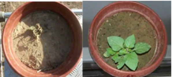
Fig. 3: Black nightshade before and after microwave
application
Fig. 4: Johnson Grass before and after microwave
application
Fig. 5: Bermuda grass before and after microwave
application
Application of Microwaves for Weed Control / Int. J. Agric. Biol., Vol. 20, No. 5, 2018
Cocklebur (X. strumarium)
As for cocklebur’s (X. strumarium) dry weight values during its 2–4 leaves developmental periods at a 1 m s-1 feed
rate, the energy demand values were found as ED 50=1.9
kW, ED 80=2.6 kW and ED 90=3.1 kW. As for the 0.3 m s-1 feed rate, these values were ED 50=0.1 kW, ED
80=0.2 kW and ED 90=0.4 kW.
In the weed’s 6–8 leaves developmental period; at a 0.1 m s-1 feed rate, 2.1 kW of energy was required to
Table 4: Cocklebur (X. strumarium)’s fresh weights and ED 50, ED 80 & ED 90 values
Growth stage Feed rate (m s-1) Regression parameter (±SE)* ED
50 (±SE) ED80 (±SE) ED90 (±SE)
B C D 2–4 leaf 0.1 0.6 (1.4) 0.1 (5.6) 16.1 (36) 0.2 (1.6) 2.2 (4.9) 8.5 (14.3) 0.3 1.4 (5.6) 1.6 (2.9) 10.6 (11) 0.6 (3) 1.7 (1.6) 3 (4.7) 6–8 leaf 0.1 24.3 (24) 8.9 (1) 16.6 (1.2) 2.2 (2.1) 2.3 (0.9) 2.4 (0.3) 0.3 24 (17) 8.6 (0.8) 16.6 (1.2) 2.2 (1.5) 2.3(0.6) 2.4 (0.2) 10–12 leaf 0.1 0.6 (1) 1.5 (17.8) 65.5 (156) 0.1 (0.9) 1.3 (5.4) 5.4 (17.1) 0.3 1.8 (3.8) 4.4 (10.2) 34.3 (3.6) 1.4 (1) 2.9 (2.9) 4.6 (8.9)
*C: lower limit, D: upper limit, E (ED 50) dosage accounting for 50% between upper and lower limit, B: gradient of the line on slope form
Table 5: Black nightshade (S. nigrum)’s dry weights and ED 50, ED 80 & ED 90 values
Growth stage Feed rate (ms-1) Regression parameter (±SE)* ED50 (±SE) ED80 (±SE) ED90 (±SE)
B C D 2–4 leaf 0.1 9.5 (11.3) 0.5 (0.4) 4.4 (0.3) 2.9 (0.3) 3.4 (0.4) 3.7 (0.8) 0.3 6.3 (13.5) 0.1 (0.2) 4.4 (0.1) 2.1 (1.8) 2.6 (1) 2.9 (0.4) 6–8 leaf 0.1 3.9 (36.7) 7.1 (0.5) 16.6 (35) 0.2 (2) 0.3 (2.9) 0.3 (3.7) 0.3 3.3 (4.7) 4.6 (6.1) 15.9 (0.7) 3 (0.8) 4.6 (3.8) 5.9 (6.9) 10–12 leaf 0.1 0.6 (4) -1.1 (46) 19.6 (57) 0.9 (4.5) 8.6 (9) 31.7 (62) 0.3 1.5 (16) 0.3 (75) 15.6 (7.1) 2.4 (11.2) 6.1 (9) 10.6 (22)
*C: lower limit, D: upper limit, E (ED 50) dosage accounting for 50% between upper and lower limit, B: gradient of the line on slope form
Table 6: Johnson grass (S. halepense)’s dry weights and ED 50, ED 80 & ED 90 values.
Growth stage Feed rate (m s-1) Regression parameter (±SE)* ED
50 (±SE) ED80 (±SE) ED90 (±SE)
B C D 2–4 leaf 0.1 0.9 (3) 0.6 (3.8) 13.6 (76) 0.1 (1.9) 0.7 (6) 1.7 (12) 0.3 0.5 (0.7) -1.2 (6.5) 17.5 (30) 0.1 (0.5) 1.7 (7.5) 9.6 (51) 6–8 leaf 0.1 3.4 (13.6) 1.6 (4.4) 17.9 (0.8) 1.8 (3.2) 2.7 (0.7) 3.4 (3) 0.3 2.5 (3.3) -0.9 (8.8) 17.9 (0.6) 2.7 (0.7) 4.6 (4.3) 6.4 (8.6) 10–12 leaf 0.1 5 (3) 3.1 (3) 18.1 (0.8) 3.2 (0.3) 4.3 (1) 5 (1.6) 0.3 16.7 (7.9) 3.9 (0.6) 18.1 (0.6) 3.3 (0.1) 3.6 (0.2) 3.7 (0.3)
*C: lower limit, D: upper limit, E (ED 50) dosage accounting for 50% between upper and lower limit, B: gradient of the line on slope form
Table 7: Bermuda grass (C. dactylon)’s dry weights and ED 50, ED 80 & ED 90 values
Growth stage Feed rate (m s-1) Regression parameter (±SE)* ED
50 (±SE) ED80 (±SE) ED90 (±SE)
B C 2–4 leaf 0.1 1 (0.7) 0.6 (0.6) 16.8 (26) 0.1 (0.2) 0.2 (0.6) 0.5 (1.2) 0.3 3.3 (6.7) 1(1.3) 6.5(0.5) 1.9 (0.8) 2.8 (1.4) 3.6 (3.4) 6–8 leaf 0.1 1.3 (5.8) 1.8 (5.3) 17.8 (37) 0.5 (3.4) 1.4 (3.5) 2.6 (2.6) 0.3 6.6 (9.7) 1.9 (0.6) 15.8 (0.7) 1.9 (0.6) 2.3 (0.2) 2.6 (0.4) 10–12 leaf 0.1 0.6 (0.6) 1.3 (5.6) 39 (57) 0.1 (0.3) 0.6 (2.1) 2.4(8) 0.3 3.8 (10.2) 3 (1.9) 17.7 (1) 1.8 (2.4) 2.6 (1) 3.2 (1.3)
*C: lower limit, D: upper limit, E (ED 50) dosage accounting for 50% between upper and lower limit, B: gradient of the line on slope form
Table 8: Cocklebur (X. strumarium)’s dry weights and ED 50, ED 80 & ED 90 values
Growth stage Feed rate (m s-1) Regression parameter (±SE)* ED
50 (±SE) ED80 (±SE) ED90 (±SE)
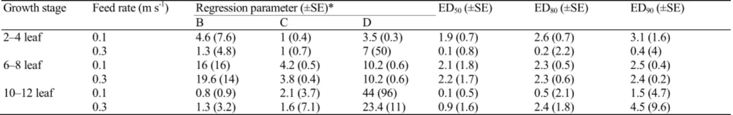
B C D 2–4 leaf 0.1 4.6 (7.6) 1 (0.4) 3.5 (0.3) 1.9 (0.7) 2.6 (0.7) 3.1 (1.6) 0.3 1.3 (4.8) 1 (0.7) 7 (50) 0.1 (0.8) 0.2 (2.2) 0.4 (4) 6–8 leaf 0.1 16 (16) 4.2 (0.5) 10.2 (0.6) 2.1 (1.8) 2.3 (0.5) 2.5 (0.4) 0.3 19.6 (14) 3.8 (0.4) 10.2 (0.6) 2.2 (1.7) 2.3 (0.6) 2.4 (0.2) 10–12 leaf 0.1 0.8 (0.9) 2.1 (3.7) 44 (96) 0.1 (0.5) 0.5 (2.1) 1.5 (4.7) 0.3 1.3 (3.2) 1.6 (7.1) 23.4 (11) 0.9 (1.6) 2.4 (1.8) 4.5 (9.6)
Kaçan et al. / Int. J. Agric. Biol., Vol. 20, No. 5, 2018 decrease dry weight by 50%, 2.3 kW of energy was
required to decrease dry weight by 80% and 2.5 kW of energy was required to decrease dry weight by 90%. When the machine’s speed was measured as 0.3 m s-1, it
was seen that the weeds could still be controlled by applying similar energy values.
During the 10–12 leaves developmental period, when the prototype machine’s feed rate was 0.1 m s-1,
the energy demand was lower in comparison to the other periods. In order to achieve 50, 80 and 90% decreases, the energy demand was 0.1, 0.5 and 1.5 kW respectively the weed’s energy demand at the 0.3 m s-1. Machine feed
rate was around two times higher while achieving a 90% decrease (Table 8).
Discussion
As we take into account the community that tested the weeds collectively formed in cotton and maize fields, we are mandated to recognize that the highest energy demand for weed control would constitute the uppermost limit. It is suggested that this projection would allow for conversion of energy and labour force. It is thus argued that to achieve effective weed control, microwave application during the early developmental periods of weeds could be exponentially beneficial. In this study at a 0.1 m s-1 feed rate
of the microwave application prototype; during the 2–4 leaves developmental periods of the weeds, an average of 1.15–4.45 kW was required to get a 80–90% decrease of weight in annual wide-leaved weeds (S. nigrum, X.
Strumarium), whilst an average of 0.3–0.45 kW was
required for perennial narrow-leaved weeds (S. halepense,
C. dactylon). Once the plants reached their 6–8 leaves
period, the energy (kW) required for 80% and 90% fresh weight shrinkage increased by around 1.5–3 times above the previous numbers. Nevertheless, for Johnson grass for instance, 2.9 kW was required for an 80% decrease and 5.8 kW was required for a 90% decrease. Once the weeds (S.
halepense) reached their 10–12 leaves developmental
periods, these energy ratios were measured as ED 80=5.5 kW and ED 90=8.7 kW, while ED 80=4.4 and ED 90=5.2 kW were reported as being effective in other weeds.
When the prototype was used with a 0.3 m s-1 feed rate
to decrease the weeds’ fresh weights during their 2–4 leaved period; 1.7 kW and 3.0 kW were needed for decreases of 80% and 90%, respectively for wide-leaved annual weeds, while these values for narrow-leaved perennial weeds were ED 80=2.3 kW and ED 90 11.8 kW. During the 6–8 leaves periods of weeds and at a feed rate of 0.3 m s-1, the energy
level required for 80% and 90% fresh weight shrinkage increased by 2–5 times. On the other hand, during the 10–12 leaved period, one of the weeds, Black nightshade (S. nigrum) required the maximum energy for 80% and 90% fresh weight shrinkage to achieve an 80% decrease. In the other weeds, respectively 3.3 kW 4.82 kW were equally effective.
As we explored the impact on weeds’ dry weights; during the 2–4 leaved period with a feed rate of 0.1 m s-1,
while decreasing dry weight by 80%, the maximum energy demand was measured in Black nightshade (S. nigrum) as 3.4 kW, while this value was found to be the maximum of 3.7 kW for a 90% decrease in the same weed. Respective energy values in the other weeds for 80% and 90% decreases were 0.7 kW and 1.7 kW for Johnson grass (S.
halepense), 0.2 kW and 0.5 kW for Bermuda grass (C. dactylon), 2.6 kW and 3.1 kW for cocklebur (X. strumarium). It was discovered that all the weeds could be
controlled by 90% with this uppermost energy limit at 3.7%. At the feed rate of 0.3 m s-1, 2.6 kW and 2.9 kW were the
values required to decrease Black nightshade’s (S. nigrum) dry weight by 80% and 90%, respectively. For another wide-leaved weed namely cocklebur, these values were measured to 0.2 and 0.4 kW. One of the perennial weeds, Johnson grass required respectively 1.7 and 9.6 kW energy for 80 and 90% shrinkage, respectively while Bermuda grass could be controlled by applying 2.8 kW and 3.6 kW of energy.
In the 6–8 leaves periods of the weeds, when the prototype was set at a 0.1 m s-1 feed rate, the energy values
required to decrease dry weights of Johnson grass by 80% and 90% were measured to be 20.7 and 3.4 kW respectively. As for other weeds, to achieve 80% and 90% reduction in weight, respectively 0.3–2.7 kW and 0.3–2.6 kW energy ranges were found to be effective. Likewise, at the feed rate of 0.3 m s-1, to decrease Johnson grass' (S.
halepense) dry matter by 80%, it was needed to apply 2.7
kW of energy, while this value was 6.4 kW for a 90% decrease and this was the maximum energy value in all the weeds investigated.
During the other 10–12 leaves period at a feed rate of 0.1 m s-1, to achieve 80% and 90% control, black nightshade
(S. nigrum) was reported as the weed requiring the
maximum energy values respectively as 8.6 kW and 31.7 kW. To decrease dry weight by 80 and 90%, other applications required energy in the range of 0.5–3.6 kW. When the prototype had a 0.3 m s-1 feed rate, in order to
achieve 80 and 90% control, S. nigrum required the maximum energy levels of 6.1 and 10.6 kW respectively. To decrease other weeds’ weights by 80%, the required energy values varied between 2.4 kW and 3.6 kW, while these values were between 3.2 kW and 4.5 kW for a 90% decrease.
This study investigated the microwave energy values which achieved decreases of 50, 80 and 90% in the dry and fresh weights of the annual wide-leaved weeds S. nigrum and X. strumarium, which cause control problems in maize and cotton fields, and the perennial weeds S. halepense and
C. dactylon. At both of the feed rates of the tested prototype
(0.1 m s-1 and 0.3 m s-1), it was found in the regression
analysis that the machine had a capacity to decrease fresh and dry weights of all weeds by ratios of 50, 80 and 90%.
Application of Microwaves for Weed Control / Int. J. Agric. Biol., Vol. 20, No. 5, 2018 leaves period were examined, it was seen that, at a feed rate
of 0.3 m s-1, in order to achieve 90% control of S. halepense
(9.6 kW), it was required to apply an approximately 3 times higher energy level than in the case of S. nigrum, C.
dactylon and X. strumarium.
At the feed rate of 0.3 m s-1, in the 6–8 leaves period
of the weeds, in order to achieve a 90% reduction of the dry weights, it was required to apply a 3 times higher energy level in S. nigrum and S. halepense in comparison to the other weeds (C. dactylon, X. strumarium). However, as manifested by other researchers as well ( Zanche et al., 2003; Sartorato et al., 2006; Cicatelli et al., 2015; Sahin and Saglam, 2015; Aygun et al.,2016) it was revealed that it could be feasible to control weeds via microwave applications by applying lower energy levels.
As for S. nigrum’s 10–12 leaves growth period and S.
halepense’s 2–4 and 6–8 leaves growth periods, the energy
levels (10.6–31.7, 11.8–12.3 kW) required to decrease their fresh and dry weights by a ratio of 90% were measured to be extremely high. The reason for this revelation could be explained through the interrelation between plant size and microwave energy as stated here: “In parallel with the widened size of plants, there will be an increase in the expansion area of microwaves; hence wave absorption of plants will correspondingly rise in an identical ratio (Wolf et al., 1993).
Particularly, herbicide-resistant weeds, invasive weeds and perennial woody weeds are promoted, and they get to have a dense population when mechanical or flame burning weed control is used (Butler, 1984). This is because these control methods miss weed seeds or root parts in the soil. In particular, the flame-burning method depends on the moisture and nutrient content of the weeds, and it depends on weather conditions. In addition, the seeds live longer in the soil (McFadyen, 1992). Besides, in pre-emergence, the main factor reducing microwave efficiency for weed control is the interaction with soil water, which substantially absorbs the microwave flux penetrating the soil. Moreover, even with low soil water content, this is expected not to be beneficial because it simply results in deeper penetration in the soil (Nelson, 1996).
However, when applied directly to weed seedlings, microwave applications do not cause adverse effects to soil nutrients and plant nutrient content. There are also safety implications for operators and passers-by regarding exposure to microwaves (Diprose et al., 1984). In our experiments, the soil moisture during treatment was 10– 12% (V/V) in the 0–15 cm top soil layer. The weeds in the pots were not irrigated for 5 days after the application. The soil temperature in all pots was measured after the application and it had increased by an average of 0.8°C.
In flame-burning tests, 108 kJ was the energy level required to achieve ED 95 in the fresh weight ratio of
Sinapis alba L.’s at two true-leaves period, while during its
6 leaves period, the energy requirement increased to 410 kJ (Ascard, 1994). The same researcher obtained similar
findings during year 1995 and 1998 tests. As we examined the hot water method, it was seen that in order to heat the soil and control weeds more effectively, a higher amount of energy is required (Melander and Jørgensen, 2005; De Cauwer et al., 2014).
Compared to the former studies in which 30–40% efficiency ratios could be measured at the analyses aimed to check the weed reserves of the soil, more current studies unveiled that via application directly on the sprouting terminal of weeds, it is easier to control weeds more effectively; hence, unlike other physical methods, the adversities could be removed and microwave applications could provide an alternative solution against the herbicide method.
That being reported, the EPPO principles stated that herbicide and control applications in post emergence weed control methods should be conducted at times when the preliminary real leaf emerges, or second real leaves become visible. Of all the applications covered in our study, ED 90 weed control values required for an effective control during the 2–4 and 6–8 leaves periods were easily obtained at energy values of 2.4, 3.2 , 4.8 and 5.6 kW at the 0.1 and 0.3 m s-1 speed values generated by
the prototype machine we designed. It has thus been posited in this study that, for weed control, it is suggested to combine microwave applications into integrated weed management systems.
Conclusion
This study clearly showed that microwaves radiation could provide control of weeds in cotton and maize fields. While use of herbicides in agriculture has a strong environmental negative impact, microwaves treatment could be also provide non-chemical control of weeds. Furthermore, it is possible to state that the prototype machine for weed control can be important to reduce costs. Moreover, the prototype machine can be easily adapted to different agricultural crops cultivation.
Acknowledgements
The Ministry of Science, Industry and Technology of Turkey supported this research.
References
Aygun, I., E. Cakir and K. Kacan, 2016. Possibilities of killing weeds by microwave power. J. Agric. Machin. Sci., 12: 285–288
Ascard, J., 1994. Dose response models for flame weeding in relation to plant size and density. Weed Res., 34: 377–385
Barker, A.V. and L.E. Craker, 1991. Inhibition of weed seed germination by microwaves. Agron. J., 83: 302‒305
Beveridge, L.E. and R.E. Naylor, 1999. Options for organic weed control - what farmers do. In: Proc. Brighton Crop Prot. Confer. – Weeds, pp: 939–944. UK British Crop Protection Council, Brighton, UK Bond, W. and A.C. Grundy, 2001. Non-chemical weed management in
Kaçan et al. / Int. J. Agric. Biol., Vol. 20, No. 5, 2018 Brodie, G., G. Harris, L. Pasma, A. Travers, D. Leyson, C. Lancaster and J.
Woodworth, 2009. Microwave soil heating for controlling ryegrass seed germination. Trans. Amer. Soc. Agric. Biol. Eng., 52: 295–302 Butler, J.E., 1984. Longevity of Parthenium hysterophorus L. seed in the
soil. Aust. Weeds, 3: 6
Cicatelli, A., F. Guarino, S. Castiglione, M. Grimaldi, A. Di Luca, D. Esposito and B. Bisceglia, 2015. Microwave treatment of agricultural soil samples. Evaluation of effects on soil quality and seed germ inability. Preliminary results. Available at: http://ieeexplore.ieee.org/stamp/stamp.jsp?tp=&arnumber=7375453 (Accessed: 20 March 2017)
Davis, F.S., J.R. Wayland and M.G. Merkle, 1973. Phytotoxicity of a UHF Electromagnetic Field. Nature, 241: 291–292
Davis, F.S., J.R. Wayland and M.G. Merkle, 1971. Ultrahigh-frequency electromagnetic fields for weed control: Phytotoxicity and selectivity. Science, 173: 535–537
De Cauwer, B., S. Bogaert, S. Claerhout, R. Bulcke and D. Reheul, 2014. Efficacy and reduced fuel use for hot water weed control on pavements. Weed Res., 55: 195–205
Diprose, M.F., F.A. Benson and A.J. Willis, 1984. The effect of externally applied electrostatic fields, microwave radiation and electric currents on plants and other organisms with special reference to weed control. Bot. Rev., 50: 171–223
Kacan, K. and O. Boz, 2014. Investigation of alternative weed management methods in organic vineyards of the aegean region. Turk. J. Agric. Nat. Sci. Special Issue, 2: 1369–1373
Knezevic, S.Z. and S.M. Ulloa, 2007. Flaming: potential new tool for weed control in organically grown agronomic crops. J. Agric. Sci., 52: 95– 104
Melander, B. and M.H. Jørgensen, 2005. Soil steaming to reduce intra row weed seedling emergence. Weed Res., 45: 202–211
McFadyen, R.E., 1992. Biological control against parthenium weed in Australia. Crop Prot., 11: 400–407
Nelson, S.O., 1996. A Review and Assessment of Microwave Energy for Soil
Treatment to Control Pests. Available
at:https://naldc.nal.usda.gov/download/34201/PDF (Accessed: 20 March 2017)
Oerke, E.C., 2006. Crop losses to pests. J. Agric. Sci., 144: 31–43 Owen, M., M. Walsh, R. Llewellyn and S. Powles, 2007. Widespread
occurrence of multiple herbicide resistance in Western Australian annual ryegrass (Lolium rigidum) populations. Aust. J. Agric. Res., 58: 711–718
Sahin, H. and R. Saglam, 2015. A research about microwave effects on the weed plants. ARPN J. Agric. Biol. Sci., 10: 81–83
Sartorato, I., G. Zanin, C. Baldoin and C. De Zanche, 2006. Observations on the potential of microwaves for weed control. Weed Res., 46: 1–9 Seefeldt, S.S., J.E. Jensen and E.P. Fuerst, 1995. Log-logistic analysis of
herbicide dose response relationships. Weed Technol., 9: 218–227 Streibig, J.C., M. Rudemo and J.E. Jensen, 1993. Dose response curves and
statistical models. In: Herbicide Bioassay, pp: 29–55. Streibig, J.C. and P. Kudsk (eds.). CRC Press, Boca Raton, Florida, USA Wayland, J., M. Merkle, F. Davis, R.M. Menges and R. Robinson, 1975.
Control of weeds with UHF electromagnetic fields. Weed Res., 15: 1–5
Wolf, W.W., C.R. Vaughn, R. Harris and G.M. Loper, 1993. Insect radar cross-section for aerial density measurement and target classification. Trans. Amer. Soc. Agric. Biol. Eng., 36: 949–954
Zanche, C.D., C. Baldoin, F. Amistà, L. Giubbolini and S. Beria, 2003. Design, construction and preliminary tests of a microwave prototype for weed control. Riv. di Ingeg. Agric., 34: 31–38