Efficient computation of joint fractional Fourier domain signal representation

(1)

Efficient computation of joint fractional Fourier

domain signal representation

Lutfiye Durak,1,*Ahmet Kemal Özdemir,2and Orhan Arikan3 1

Department of Electronics and Communications Engineering, Yildiz Technical University, Besiktas, Istanbul 34349, Turkey

2

WesternGeco AS, Schlumberger House/Solbraavein 23, Asker 1383, Norway

3

Department of Electrical Engineering, Bilkent University, Ankara 06800, Turkey *Corresponding author: lutfiye@ieee.org

Received August 3, 2007; revised December 19, 2007; accepted January 9, 2008; posted January 10, 2008 (Doc. ID 86062); published February 21, 2008

A joint fractional domain signal representation is proposed based on an intuitive understanding from a time-frequency distribution of signals that designates the joint time and time-frequency energy content. The joint tional signal representation (JFSR) of a signal is so designed that its projections onto the defining joint frac-tional Fourier domains give the modulus square of the fracfrac-tional Fourier transform of the signal at the corresponding orders. We derive properties of the JFSR, including its relations to quadratic time-frequency representations and fractional Fourier transformations, which include the oblique projections of the JFSR. We present a fast algorithm to compute radial slices of the JFSR and the results are shown for various signals at different fractionally ordered domains. © 2008 Optical Society of America

OCIS codes: 070.0070, 070.2575.

1. INTRODUCTION

One of the major areas of research in time-frequency sig-nal processing is the design of novel time-frequency rep-resentations that are utilized to analyze and process non-stationary signals [1,2]. As time-frequency distributions do not always convey desirable qualifications in every ap-plication, the demand for powerful signal representations has led to a substantial amount of research on the design of 2D signal representations defined by alternative vari-ables other than time and frequency. Joint time-scale rep-resentations, which have attracted much interest espe-cially in the fields of sonar and image processing, constitute one of the earliest examples of this type of rep-resentation. Other popular choices of joint variables in-clude higher derivatives of the instantaneous phase of signals for radar and sonar problems [3,4]; dispersive time-shifts for wave propagation problems and analogs of quantum mechanical quantities such as spin, angular mo-mentum, and radial momentum [5]; and scale-hyperbolic time, warped time-frequency, and warped time-scale. Such signal representations have been derived by using two alternative approaches that are both based on the op-erator theory: the variables are associated with either Hermitian operators as in [2] or unitary operators as in [5]. Similarly, a joint fractional signal representation has been derived in a mathematical framework by associating Hermitian fractional operators to fractional Fourier transform (FrFT) variables constituting the joint distribu-tion [6].

The fractional Fourier domains are the set of all do-mains interpolating between time and frequency [7,8]. The associated transform, FrFT with order a transforms a signal into the ath-order fractional Fourier domain and the ath-order FrFT of x共t兲 is given by [9]

xa共t兲 ⬅ 兵Fax其共t兲 =

冕

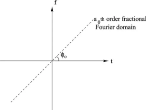
Ba共t,t⬘兲x共t⬘兲dt⬘, − 2⬍ a ⬍ 2, 共1兲 where Ba共t,t⬘兲 = e−j共␲ sgn共a兲/4+␾/2兲 兩sin␾兩1/2 e j␲共t2_cot_␾−2tt_⬘_csc_␾+t_⬘2_cot_␾兲共2兲 is the transformation kernel,␾=a共␲/2兲 and sgn共兲 is the sign function.

The fractional Fourier domains corresponding to a = 0 and 1 are the time and frequency domains, respectively. The FrFT with an order parameter a = a0 transforms a

signal into the a0th-order fractional Fourier domain,

which is oriented by ␾0= a0␲/2 with respect to the time

axis in the counterclockwise direction as illustrated in Fig. 1. The FrFT has found many applications in signal processing [10–16], optics, diffraction theory, optical propagation, and optical signal processing [17–20].

In this paper, we derive the joint fractional signal rep-resentation (JFSR), which designates the energy contents of signals in fractional Fourier domain variables instead of time and frequency. To this end, rather than using cum-bersome mathematical equations based on operator theory, we extend our intuitive understanding from a time-frequency distribution, i.e., a function that desig-nates joint time and frequency contents of signals. Then, we derive some important properties of the JFSR includ-ing its relation to quadratic time-frequency representa-tions and fractional Fourier transformarepresenta-tions, and present a simple formula for its oblique projections. We also present a fast algorithm to compute radial slices of the JFSR and numerically computed JFSRs of some synthetic signals.

(2)

The outline of the paper is as follows. In Section 2, a concise derivation of JFSR is presented and some of its properties are provided. After presenting a fast computa-tion algorithm in Seccomputa-tion 3, JFSRs of some synthetic sig-nals are numerically computed in Section 4. Finally, con-clusions are drawn in Section 5.

2. DISTRIBUTION OF SIGNAL ENERGY ON

JOINT FRACTIONAL FOURIER

DOMAINS

One of the primary expectations from a time-frequency distribution Dx共t,f兲 associated with a signal x共t兲 is that it

An-other nice property of the WD is that its oblique

projec-tions give the energy distribution with respect to the

cor-responding fractional Fourier domain [21]. Such

properties and its ability to provide high time-frequency domain signal concentration make the WD attractive compared to other representations. Although the WD and its enhanced versions are useful in time-frequency analy-sis, in some applications such as signal design and syn-thesis it is more useful to have a time-fractional Fourier domain representation.

In this section, the JFSR is constructed using condi-tions similar to the ones given in Eqs.(3)–(5). The JFSR is then generalized to a cross JFSR, and some properties of the JFSR are investigated in detail.

A. JFSR

Let the JFSR of a signal be denoted by Exa共u,v兲 where a

=共a1, a2兲 denotes the orders of fractional Fourier domains

u and v, respectively. It is desired that the marginal den-sities satisfy

冕

Exa共u,v兲dv = 兩xa1共u兲兩

2_, _共7兲

冕

Exa共u,v兲du = 兩xa₂共v兲兩2, 共8兲

where兩xa₁共u兲兩2and兩xa₂共v兲兩2are the energy contents of the

signal at the a1th and a2th fractional Fourier domains,

re-spectively. Similar to Eq.(5), the overall integral on the u – v plane is desired to be

冕冕

Exa共u,v兲dudv = 储x储2. 共9兲

The conditions stated in Eqs. (7)–(9) make the JFSR a generalization of the WD, since the JFSR reduces to the WD when共a1, a2兲=共0,1兲.

To construct the distribution Ex a

共u,v兲 satisfying the con-ditions on the marginal densities and the total energy, we make use of the projection property of the WD [21]:

冕

Wx共u cos␾ − v sin ␾,u sin ␾ + v cos ␾兲dv = 兩xa共u兲兩2.

共10兲 In Fig.2, we observe that the value of the time-frequency distribution at a point P contributes to the energy densi-ties of the fractional Fourier domains u and v at points u = u0 and v = v0, respectively. Therefore, the JFSR can

simply be formed by redistributing the WD so that Exa共u,v兲 = CWx共P共t共u,v兲,f共u,v兲兲兲, 共11兲

where the coordinates_{共u,v兲 and 共t,f兲 are related by}

冋

cos␾1 sin␾1 cos␾2 sin␾2

册冋

t f

册

=

冋

u v

册

, 共12兲

and ␾i= ai␲/2 for i=1,2. By using the total energy

con-straint [Eq.(9)], the constant C in Eq.(11)is determined as

Fig. 1. a0th-order fractional Fourier domain makes an angle of

(3)

C =兩csc共␾12兲兩, 共13兲

where␾12=␾2−␾1. Thus, Exa共u,v兲 is explicitly given by

− j2␲␶− u cos␾2+ v cos␾1

sin␾12

冊

d␶. An equivalent and more compact form of Exa共u,v兲 can be

obtained by using the rotation effect of the FrFT on the WD,

Wx_a

1共u,v兲 = Wx共u cos␾12

− v sin␾12,u sin␾12+ v cos␾12兲,

_{u −}␶ sin ␾12 2

冊

⫻ e−j2␲共v−u cos␾12兲␶_d␶. 共16兲

Defining Exa共u,v兲 through its relation to the WD

pro-vides an easily interpretable definition of the JFSR of

sig-nals. From the definition given in Eq.(15), it follows that JFSR is a quadratic distribution while it is not a time-frequency distribution. Therefore it belongs to a broader class than the familiar Cohen’s class. Thus, its introduc-tion to the nonstaintroduc-tionary signal processing will bring new insights into the design, filtering, analysis, and synthesis of signals in many applications.

C. Properties of the JFSR

In this section, we investigate the properties of the JFSR. In the properties listed below, the joint fractional Fourier domains have the orders of a =共a1, a2兲 making angles of

共␾1,␾2兲 with respect to the time axis where␾i= ai共␲/2兲.

Property 1. The JFSR is a real distribution

Exa共u,v兲 = 共Exa兲*共u,v兲. 共17兲

Property 2. The orthogonal projections of the JFSR of a signal x共t兲 onto u and v axes give the magnitude square of the FrFTs of the signal at orders associated with these axes, that is,

冕

Exa共u,v兲dv = 兩xa1共u兲兩

2_, _共18兲

冕

Exa共u,v兲du = 兩xa2共v兲兩

2_. _共19兲

Property 3. The area under the JFSR of a signal x共t兲 gives the total signal energy

冕冕

Exa共u,v兲dudv =

冕

兩x共t兲兩2dt, 共20兲

which follows from Property 2 and the unitarity of the FrFT.

Property 4. The JFSR and WD of a signal x共t兲 are re-lated as Exa共u,v兲 = 兩csc␾12兩Wxa₁

冉

Property 6. Any oblique projection of JFSR of a signal x_{共t兲 onto an oblique axis making an angle of}␾ is

P_␾关E_xa兴共r兲 = 兩x_共a_⬘_兲共r/M兲兩2_, _a_⬘₌2␾⬘

␲ , 共22兲

where

␾⬘= arctan 2共cos␾1+ cos␾ + cos ␾2sin␾,sin ␾1cos␾

+ sin␾2sin␾兲, 共23兲

M =共1 + sin 2␾ cos ␾12兲1/2. 共24兲

Proof: By the projection-slice theorem, the oblique

pro-jection of the JFSR of x共t兲 at an angle␾ is given by P_␾关E_xa兴共r兲 =

冕

Fx共␨ cos␾,␨ sin ␾兲e−j2␲␨rd␨, 共25兲

where

Fxa共␨,␩兲 =

冕冕

Exa共u,v兲ej2␲共␨u+␩v兲dudv, 共26兲

is the radial slice of the 2D inverse Fourier transform of the JFSR of x共t兲. By using Eq.(21), the following expres-sion can be obtained for F_x共a兲共␨,␩兲 in terms of the ambigu-ity function Ax共兲 of x共t兲

Fxa共␨,␩兲 = Ax共␨ cos␾1+␩cos␾2,␨ sin␾1+␨ sin␾2兲.

共27兲 Thus, the radial slice Fx

a

共␨ cos␾,␨ sin ␾兲 of Fx a

共␨,␩兲 can be expressed as

F_xa共␨ cos␾,␨ sin ␾兲 = Ax共␨M cos␾⬘,␨M sin␾⬘兲, 共28兲

where␾

⬘

and M are as given in Eqs.(23)and(24), respec-tively. It is known that the radial slice of the ambiguity function of a signal x共t兲 at the angle␾ has the following relation to the共a

⬘

兲th FrFT of the signal x共t兲

Ax共␨ cos␾⬘,␨ sin␾⬘兲 =

冕

兩x共a_⬘兲共r兲兩2ej2␲␨rdr. 共29兲

Then, the relation in Eq.(22)can be obtained by

combin-ing Eqs.(25),(28), and(29). 䊏

Property 7. Similar to the time-bandwidth product analysis on the joint time-frequency plane, the product of the spreads of signals in arbitrary fractional Fourier do-mains can also be defined. In [9], it has been shown that the product of the spreads of a signal x共兲 in two arbitrary

fractional Fourier domains a1and a2are bounded below

by

␴a1␴a2ⱖ

兩sin关␲共a1− a2兲/2兴兩

4␲ , 共30兲

where␴a_1,2is defined as follows:

␴a_1,2=

冋

冕

共ua_1,2−␩a_1,2兲2兩xa_1,2共ua_1,2兲兩2dua_1,2

册

1/2

冒

储x储,

共31兲 ␩a_1,2=

冋

冕

ua_1,2兩xa_1,2共ua_1,2兲兩2dua_1,2

册

冒

储x储2, 共32兲

where ua_1,2represents the a1,2th-order fractional Fourier

domains. In [22], a tighter lower bound is derived for real signals, and it is shown that this bound actually corre-sponds to the product of fractional domain spreads of a Gaussian function. The analysis on the fractional domain spreads indicates that, as the joint parameters vary, the product of the spreads and consequently the area of the support of the signals on the joint fractional plane varies, and it diminishes to 0 as the joint fractional Fourier order parameters are equal to each other.

3. FAST COMPUTATION OF THE JFSR

In this section, we provide an efficient computation algo-rithm of the JFSR of a signal on arbitrary radial slices. Throughout the computations, we assume that the signal x共t兲 is scaled to x共t/s兲 before sampling, so that its WD is approximately confined into a circle of radius⌬x/ 2. Here,

if the time width and bandwidth of the signal is approxi-mately⌬tand⌬f, respectively, then the scaling parameter

s becomes s =共⌬f/⌬t兲1/2providing a signal that has

negli-gible energy outside the interval关−⌬x/ 2 ,⌬x/ 2兴.

To compute the radial slice of the JFSR of a signal x共t兲, we use the relation

Exa

a_{共r cos}_{␾,r sin ␾兲 = 兩csc ␾}

12兩Wx共r cos␾⬘,r sin␾⬘兲,

共33兲 where

␾⬘= arctan共cos␾ cos ␾2+ sin␾ cos ␾1,cos␾ sin ␾2

− sin␾ cos ␾1兲, 共34兲

and ␾1 and ␾2 are the corresponding angles of the

frac-tional Fourier domains u and v with respect to the time axis. It has been shown in [15] that the radial slice of the WD along the line共r cos␾

⬘

, r sin␾

⬘

⫻共k/共2⌬x兲兲 is computed using the algorithm given in [23]

with O共N log N兲 computational complexity.

As the relationship [Eq.(36)] depends on the FrFTs of the signal x共t兲, computation of any M uniformly spaced samples on the line segment r苸关ri, rf兴 along the radial

slice of E_x

a

a_共r⌬

xcos␾,r⌬xsin␾兲 can be performed through

the chirp-z transform algorithm in O共共N+M兲log共N+M兲兲

computational complexity [24]. In Section 4, the results of the algorithm are presented for synthetic signals on vari-ous joint fractional Fourier planes.

4. SIMULATIONS

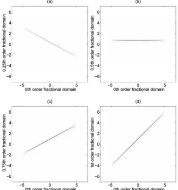
In this section, the JFSR of a chirp signal and a quadratic FM modulated signal that has a nonconvex time-frequency support on the time-time-frequency plane are evalu-ated for four different joint fractional Fourier order pairs of a =共a1, a2兲 as 共0,0.25兲, 共0,0.5兲, 共0,0.75兲, and 共0,1兲.

Moreover, an application example, which makes use of the localization property of the JFSR is presented by em-ploying the time-frequency component analyzer algorithm in [25].

For a chirp signal of x共t兲=rect共t/10兲exp共j2␲共0.5t2_{+ t}_兲兲,

the JFSRs of the four different a =_共a1, a2兲 are presented in

Fig.3. The distribution given in Fig.3(d)is the same as the WD of x共t兲 because the fractional order parameters of the domains are a1= 0, a2= 1, corresponding to the time

and frequency domains, respectively. As shown in Fig.3, the supports of the chirp signal at various joint fractional Fourier planes remains linear. However, the localization of the resultant components varies, because the uncer-tainty relation of the fractional Fourier domains has a tighter lower-bound when compared to the time and fre-quency domains [9].

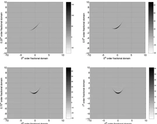
The JFSRs of a quadratic FM modulated signal x共t兲

= exp共−␲共共t/3兲2_{+ 0.3jt}3_{兲兲, which has a nonconvex}

time-frequency support on the time-time-frequency plane are pre-sented in Fig.4. The distribution given in Fig.4(d)with fractional Fourier order pair_{共0,1兲 is the same as the WD} of x共t兲. It is easier to observe the localization of the signal component that depends on the order of the joint frac-tional Fourier domains. By comparing Figs.4(a)and4(d), it will be noticed that the amount of cross-term interfer-ence is significantly less when the two fractional orders are closer to each other. We expect that these types of

properties of JFSR will facilitate the analysis and design of time-frequency distributions where the signal compo-nents have curved time-frequency supports.

We also compute the JFSR of a 2.5 ms echolocation pulse emitted by a large brown bat, eptesicus fuscus. The recorded signal is plotted in Fig. 5(a)and can be down-loaded at [26]. The time axis in Fig.5(a)has been scaled as discussed in [23]. Figures5(b)–5(d)show the JFSR of the bat signal that has been evaluated for three different joint fractional Fourier order pairs of a =共a1, a2兲 as 共0,1兲,

共0,1.2兲, and 共0,1.3兲. The distribution given in Fig.5(b)is the same as the WD, because the fractional order param-eters a1= 0 and a2= 1 correspond to the time and

fre-quency domains, respectively. We see that the bat signal is composed of several components with nonconvex time-frequency supports. Therefore, the WD contains both in-ner and outer interference terms. In each of the plots, Figs.5(c)and5(d), one of the components in the bat signal has a very localized fractional frequency content. This is consistent with the fact that the uncertainty relation of the fractional Fourier domains has a tighter lower-bound when compared to the time and frequency domains [9].

Because of its localization property, the JFSR can be used to compute the instantaneous fractional frequency content of the analyzed signals. This will be illustrated on the signal shown in Fig.6(a), which is one of the compo-nents extracted from the bat signal given in Fig.5(a)by using the time-frequency component analyzer algorithm [25]. Figure6(b)shows the WD of the component and Fig. 6(c)shows its JFSR corresponding to the fractional Fou-rier order pairs of共0,1.2兲. In this domain, the analyzed

component contains only a very narrow band of

a2= 1.2th-order fractional frequency. Here we extend the

definition of instantaneous frequency to the fractional do-main as follows:

Fig. 3. JFSRs of x_{共t兲=rect共t/10兲e}j2␲共0.5t2_+t兲

at joint fractional Fou-rier domains with orders (a) 共a1, a2兲=共0,0.25兲, (b) 共a1, a2兲

(6)

Fig. 5. (a) 2.5 ms echolocation pulse emitted by a large brown bat, eptesicus fuscus. The JFSRs at joint fractional Fourier domains with orders (b)_共a₁, a₂_{兲=共0,1兲, (c) 共a}₁, a₂_{兲=共0,1.2兲, (d) 共a}₁, a₂_{兲=共0,1.3兲.}

Fig. 4. JFSRs of x共t兲=e−␲共共t/3兲2+0.3jt3兲 _{at joint fractional Fourier domains with orders (a)} _共a

1, a2兲=共0,0.25兲, (b) 共a1, a2兲=共0,0.5兲, (c)

(7)

fa1,a2共u兲 =

冕

−⬁ ⬁ vWa1,a2共u,v兲dv

冕

−⬁ ⬁ Wa1,a2共u,v兲dv , 共38兲

which is the center of mass of the JFSR along the v axis. The plot Fig.6(d)shows the computed instantaneous fre-quency from the JFSR shown in Fig.6(c). Essentially, this is the a2th-order fractional frequency content in the

sig-nal xa₁共u兲.

5. CONCLUSIONS

A joint fractional domain signal representation is devel-oped using the energy density interpretation of the WD on the time-frequency plane. The共u,v兲 axes defining the joint representation are chosen as the a =共a1, a2兲th-order

fractional Fourier domains. The distribution is designed so that its projections onto the u and v axes gives the modulus square of the fractional Fourier transform of sig-nals at the corresponding orders a1and a2as兩xa₁共t兲兩2and

兩xa₂共t兲兩2, respectively. It is shown that the distribution

Exa共u,v兲 depends on the WD through a coordinate

trans-formation. Therefore, the JFSR is a real-valued distribu-tion, too. The overall integral of the JFSR on the共u,v兲 plane gives the total energy of the signal. In this paper, as

part of the novel results, oblique projections of the JFSR is also derived, and a fast computation algorithm de-signed for the computation of arbitrary radial slices of the WD in [15] is extended to the computation of the JFSR. The JFSRs of various signals at various fractionally or-dered domains are presented, and the localization of the signal components are compared.

The JFSR is not analyzed in the framework of the fa-miliar Cohen’s class. Therefore, its introduction to the nonstationary signal processing will bring new insights into the design, filtering, analysis, and synthesis of signals.

ACKNOWLEDGMENTS

We thank Curtis Condon, Ken White, and Al Feng of the Beckman Institute of the University of Illinois for the bat data and for permission to use it in this paper.

REFERENCES

1. F. Hlawatsch and G. F. Boudreaux-Bartels, “Linear and quadratic time-frequency signal representations,” IEEE Signal Process. Mag. 9, 21–67 (1992).

2. L. Cohen, Time-Frequency Analysis (Prentice Hall, 1995). 3. S. Mann and S. Haykin, “The chirplet transform: physical Fig. 6. (a) One of the components extracted from the bat signal. (b) The WD of the component and (c) its JFSR corresponding to the fractional Fourier order pairs of共0,1.2兲. (d) The computed instantaneous frequency from the JFSR shown in (c).

(8)

considerations,” IEEE Trans. Signal Process. 43,

2745–2761 (1995).

4. R. G. Baraniuk and D. L. Jones, “Matrix formulation of the chirplet transform,” IEEE Trans. Signal Process. 44, 3129–3135 (1996).

5. R. G. Baraniuk, “Beyond time-frequency analysis: energy density in one and many dimensions,” IEEE Trans. Signal Process. 46, 2305–2314 (1998).

6. O. Akay and G. F. Boudreaux-Bartels, “Joint fractional signal representations,” J. Franklin Inst. 337, 365–378 (2000).

7. L. B. Almedia, “The fractional Fourier transform and time-frequency representations,” IEEE Trans. Signal Process.

42, 3084–3091 (1994).

8. H. Ozaktas and O. Aytür, “Fractional Fourier domains,” Signal Process. 46, 119–124 (1995).

9. H. M. Ozaktas, Z. Zalevsky, and M. A. Kutay, The

Fractional Fourier Transform with Applications in Optics and Signal Processing (Wiley, 2000).

10. H. M. Ozaktas, B. Barshan, D. Mendlovic, and L. Onural, “Convolution, filtering, and multiplexing in fractional Fourier domains and their relation to chirp and wavelet transforms,” J. Opt. Soc. Am. A 11, 547–559 (1994). 11. B. Barshan, M. A. Kutay, and H. M. Ozaktas, “Optimal

filtering with linear canonical transformations,” Opt. Commun. 135, 32–36 (1997).

12. M. A. Kutay, H. M. Ozaktas, O. Arikan, and L. Onural, “Optimal filtering in fractional Fourier domains,” IEEE Trans. Signal Process. 45, 1129–1143 (1997).

13. M. A. Kutay and H. M. Ozaktas, “Optimal image restoration with the fractional Fourier transform,” J. Opt. Soc. Am. A 15, 825–833 (1998).

14. M. F. Erden and H. M. Ozaktas, “Synthesis of general linear systems with repeated filtering in consecutive fractional Fourier domains,” J. Opt. Soc. Am. A 15, 1647–1657 (1998).

15. A. K. Özdemir and O. Arikan, “Efficient computation of the

ambiguity function and the Wigner distribution on arbitrary line segments,” IEEE Trans. Signal Process. 49, 381–393 (2001).

16. L. Durak and O. Arikan, “Short-time Fourier transform: two fundamental properties and an optimal implementation,” IEEE Trans. Signal Process. 51,

1231–1242 (2003).

17. V. Namias, “The fractional order Fourier transform and its application to quantum mechanics,” J. Inst. Math. Appl. 25, 241–265 (1980).

18. L. M. Bernardo and O. D. D. Soares, “Fractional Fourier transform and optical systems,” Opt. Commun. 110, 517–522 (1994).

19. H. M. Ozaktas and D. Mendlovic, “Fractional Fourier optics,” J. Opt. Soc. Am. A 12, 743–751 (1995).

20. O. Aytür and H. Ozaktas, “Non-orthogonal domains in phase space of quantum optics and their relation to fractional Fourier transform,” Opt. Commun. 120, 166–170 (1995).

21. A. W. Lohmann and B. H. Soffer, “Relationships between the Radon–Wigner and fractional Fourier transforms,” J. Opt. Soc. Am. A 11, 1798–1801 (1994).

22. S. Shinde and V. M. Gadre, “An uncertainty principle for real signals in the fractional Fourier transform domain,” IEEE Trans. Signal Process. 49, 2545–2548 (2001). 23. H. M. Ozaktas, O. Arikan, M. A. Kutay, and G. Bozdagi,

“Digital computation of the fractional Fourier transform,” IEEE Trans. Signal Process. 44, 2141–2150 (1996). 24. L. R. Rabiner, R. W. Schafer, and C. M. Rader, “The chirp

z-transform algorithm and its applications,” Bell Syst.

Tech. J. 48, 1249–1292 (1969).

25. A. K. Ozdemir, S. Karakas, E. D. Cakmak, D. I. Tufekci, and O. Arikan, “Time-frequency component analyzer and its application to analysis of brains oscillatory activity,” J. Neurosci. Methods 145, 107–125 (2005).

26. http://www.dsp.rice.edu/software/TFA/RGK/BAT/ batsig.bin.Z.